Impact-Echo Testing
Impact-Echo is a stress-wave nondestructive testing method where a short-duration mechanical impact on a concrete surface generates stress waves that reflect fr...
32 min read
Non-Destructive Testing
Concrete NDT
+4
Acoustic Emission (AE) is a passive non-destructive testing method that detects and locates transient stress waves generated by active defect processes — crack growth, corrosion, fiber breakage, and tendon wire fracture — in real time. Used for continuous bridge monitoring, pressure vessel hydrotesting, and structural health monitoring systems.
Acoustic Emission (AE) is the phenomenon of transient elastic wave generation resulting from the rapid release of localized strain energy within a material under stress. Per ASTM E1316-24 (Standard Terminology for Nondestructive Examinations, Section B), AE is defined as “the class of phenomena whereby transient elastic waves are generated by the rapid release of energy from localized sources within a material, or the transient elastic waves so generated.” This definition establishes AE as both the physical process and the measurable signal that propagates from defect activity.
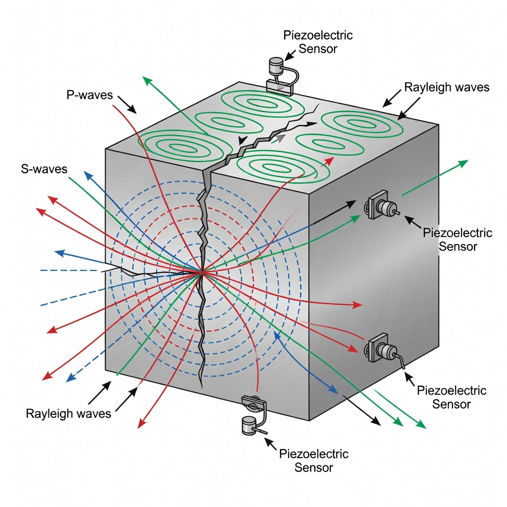
The physical mechanism operates as follows: when a material is subjected to applied stress, localized regions undergo irreversible deformation mechanisms — dislocation movement (slip), micro-yielding, twinning, inclusion fracture, grain boundary sliding, martensitic phase transformation, and crack initiation or propagation. Each such event releases a portion of the stored elastic strain energy as a stress wave packet that propagates through the material in multiple wave modes: longitudinal P-waves (compression), shear S-waves (transverse), surface Rayleigh waves, and guided Lamb waves in plate-like geometries. Source durations range from sub-microsecond for dislocation avalanches to several milliseconds for gross yielding or fiber bundle failure in composites. The generated stress waves propagate at material-specific velocities — approximately 5900 m/s for P-waves in steel, 3100 m/s for S-waves in steel, 4100 m/s for P-waves in concrete, and 2500 m/s for S-waves in concrete — with attenuation governed by geometric spreading, material absorption, and scattering at grain boundaries and interfaces.
The frequency content of AE signals spans from 20 kHz to 1 MHz for most structural monitoring applications, though specific processes produce characteristic frequency bands. Gross plastic yielding and large-scale fracture events produce lower frequencies in the 1-50 kHz range. Crack propagation in metals typically occupies 100-400 kHz. Fiber breakage in composites emits at 200-600 kHz. Hydrogen bubble formation in corrosion processes generates 100-300 kHz signals. This frequency content distinguishes AE from seismic events (0-60 Hz), audible noise (20 Hz-20 kHz), and conventional ultrasonic testing (0.5-20 MHz).
AE is classified as a passive NDT method — it does not inject energy into the structure but rather listens for energy released by the material itself during active defect processes. This is fundamentally different from active NDT methods such as ultrasonic testing (UT), impact-echo, or ground-penetrating radar (GPR), which inject energy and analyze the structural response. The passive nature of AE means that the structure must be subjected to changing stress conditions — mechanical loading, thermal cycling, or pressure changes — for damage mechanisms to emit detectable signals.
The Kaiser effect, first systematically investigated by Joseph Kaiser in 1950 during his doctoral work at the Technical University of Munich, describes the irreversible characteristic of acoustic emission behavior: when a material is loaded, unloaded, and then reloaded, acoustic emissions are absent until the previously applied maximum stress level is exceeded. This phenomenon reflects the material possessing a direct “stress memory” — once a material has been stressed to a certain level and relaxed, the microstructural adjustments (dislocation pinning, local plastic deformation) that occurred during initial loading are largely irreversible under subsequent loading until the prior stress maximum is surpassed.
Formally defined in ISO 16837:2019 (Section 3.2), the Kaiser effect is described as “little AE activity observed until the maximum load of the previous stage is surpassed when stresses are applied, removed and then reapplied to a material or a structure.” The physical explanation lies in dislocation theory: during initial loading, dislocations become pinned at obstacles (grain boundaries, precipitates, inclusions), and the AE generated comes from unpinning events and dislocation avalanches. Upon unloading and reloading, no additional dislocation unpinning occurs until the applied stress exceeds the previous maximum, enabling dislocations to overcome previously established pinning barriers.
The Kaiser effect is fundamental to AE testing methodology because it allows differentiation between new damage (emitting) and previously stabilized conditions (non-emitting). This is exploited in pressure vessel hydrotesting where the first pressurization reveals local yielding in high-stress regions while the second pressurization at the same pressure should remain acoustically quiet if the vessel is structurally sound. The effect can be nullified by several factors: temperature changes that alter residual stress states, metal fatigue from cyclic loading over operating life, creep and relaxation phenomena, corrosion damage creating new flaws at lower stress levels, and damage accumulation in composites where matrix cracking, fiber breakage, and delamination occur progressively under cyclic loading.
When the Kaiser effect is violated — AE activity resumes before reaching the previous maximum stress — the phenomenon is termed the Felicity effect, named after the research group at the University of Denver that first characterized this behavior in composite materials during the 1970s. The Felicity Ratio (FR) quantifies this effect:
[FR = \frac{\text{Load at which AE resumes}}{\text{Previous maximum load}}]
A perfectly intact structure with no damage accumulation yields an FR of 1.0, indicating perfect Kaiser effect compliance. As damage accumulates, the FR decreases — values below 0.95 indicate the presence of active damage processes requiring investigation, values below 0.90 indicate significant damage, and values below 0.80 indicate critical damage demanding immediate structural intervention. In some highly redundant, sound concrete structures, FR values can occasionally exceed 1.0 due to stress redistribution enabling new AE sources at previously unstressed locations.
Typical acceptance criteria established across ASME guidelines, ISO standards, and industry practice are:
| Felicity Ratio Range | Damage Classification | Required Action |
|---|---|---|
| FR ≥ 0.95 | Acceptable — no significant new damage | Continue normal service |
| 0.90 ≤ FR < 0.95 | Marginal — possible minor damage | Further investigation within 30 days |
| 0.80 ≤ FR < 0.90 | Significant damage present | Detailed inspection within 7 days |
| FR < 0.80 | Critical damage | Immediate shutdown and repair |
| FR > 1.05 (composites) | Stress redistribution, redundant load paths | Monitor, investigate if persistent |
ISO 16837:2019 adapts the Felicity ratio framework for reinforced concrete bridge beams using two derived parameters. The Load Ratio (L) is defined as L = L₀/Lₚ where L₀ is the load at onset of AE activity in subsequent loading and Lₚ is the previous maximum load — directly analogous to the Felicity ratio. The Calm Ratio (C) is defined as C = Aᵤ/Aₜ where Aᵤ is the cumulative AE activity during unloading and Aₜ is the total AE activity during the entire loading cycle. Sound structures show minimal AE during unloading (low calm ratio), while significantly damaged structures continue emitting even as load is removed — a behavior associated with crack face rubbing, fretting, and debris crushing during load reduction. Damage is classified per ISO 16837 into low, medium, and severe categories based on the combination of load ratio and calm ratio plotted on a standardized damage classification chart.
The primary AE source mechanisms span the full range of material deformation and damage processes. Each mechanism produces characteristic AE signatures differentiated by amplitude, frequency, duration, and energy content:
| Source Mechanism | Relative Energy | Frequency Range | Typical Amplitude (dBAE) | Typical Duration |
|---|---|---|---|---|
| Dislocation motion (microplasticity) | Very low | 100-1000 kHz | 30-50 | 1-10 μs |
| Inclusion/martensite fracture | Low | 100-500 kHz | 40-60 | 5-50 μs |
| Grain boundary sliding | Low-Medium | 50-300 kHz | 45-65 | 10-100 μs |
| Crack initiation | Medium | 50-500 kHz | 55-75 | 20-500 μs |
| Crack propagation (subcritical) | Medium-High | 50-400 kHz | 60-85 | 100-1000 μs |
| Fiber breakage (composites) | Medium | 100-600 kHz | 60-90 | 10-100 μs |
| Delamination (composites) | High | 50-300 kHz | 70-95 | 200-2000+ μs |
| Wire/tendon breakage | Very High | 5-200 kHz | 80-100+ | 1-20 ms |
| Hydrogen bubble collapse (corrosion) | Low | 100-500 kHz | 35-55 | 50-200 μs |
| Pitting corrosion | Low-Medium | 100-400 kHz | 45-70 | 10-100 μs |
| Leak-induced AE | Continuous (RMS) | Broadband | ASL 30-70 | Continuous |
| Plastic deformation (gross yielding) | High | 1-50 kHz | 70-100 | 0.1-10 ms |
AE sensors are predominantly piezoelectric devices utilizing lead zirconate titanate (PZT) ceramic elements. When a stress wave impinges on the sensor face, the piezoelectric element undergoes mechanical deformation, generating a surface charge that produces a voltage proportional to the instantaneous surface displacement velocity. The sensor output is a damped sinusoidal waveform whose characteristics encode information about the original source mechanism, propagation path, and material properties. Per ASTM E650 (Standard Guide for Mounting Piezoelectric Acoustic Emission Sensors), proper mounting with acoustic couplant is essential for consistent signal transmission and reproducible results across successive tests.
Two fundamental sensor architectures exist, each suited to different monitoring objectives:
Resonant sensors feature a PZT element designed to maximize sensitivity at a specific frequency by matching the element thickness to half the acoustic wavelength at the target frequency. A 150 kHz resonant sensor uses a PZT element approximately 12 mm in diameter and 14 mm thick. These sensors offer the highest sensitivity (typically -65 to -75 dB ref 1 V/μbar) at their resonant frequency, providing excellent signal-to-noise ratios for detecting low-energy emission events. Standard resonant frequencies include: 60 kHz for concrete and geomaterials (high attenuation), 150 kHz for general-purpose steel monitoring (bridge steel, pressure vessels, pipes), 300 kHz for fiber composites (matrix cracking and fiber breakage), and 500 kHz for laboratory materials testing. The primary limitation of resonant sensors is their narrow bandwidth — sensitivity drops sharply away from resonance, limiting the information available for frequency-based source classification.
Broadband sensors use backing materials and mechanical damping to suppress resonance, producing a relatively flat frequency response over a wide range — typically 100-1000 kHz or 50-2000 kHz for specialized models. These are essential for research applications requiring spectral analysis of AE signals, source mechanism classification based on frequency content, and material characterization studies. The trade-off is lower sensitivity compared to resonant sensors — typically -75 to -85 dB ref 1 V/μbar — making them less suitable for detecting very low-amplitude events in noisy environments. Examples include the Physical Acoustics WD (100-1000 kHz, integral preamp), the Vallen VS900-M (100-900 kHz), and the MISTRAS Micro-30S (300-700 kHz, miniature).
| Sensor Model | Type | Frequency Range | Sensitivity | Typical Application |
|---|---|---|---|---|
| R15I | Resonant | 50-200 kHz (150 kHz peak) | -65 dB | Steel bridges, pressure vessels |
| R30I | Resonant | 100-400 kHz (300 kHz peak) | -68 dB | Composite materials, FRP |
| R6I | Resonant | 30-100 kHz (60 kHz peak) | -72 dB | Concrete, masonry, rock |
| R80I | Resonant | 70-200 kHz (80 kHz peak) | -70 dB | Timber, wood structures |
| WD | Broadband | 100-1000 kHz | -78 dB | Research, multi-source classification |
| Micro-30S | Resonant | 300-700 kHz | -74 dB | Thin composites, miniature |
| VS900-M | Broadband | 100-900 kHz | -80 dB | Laboratory, spectrum analysis |
| PK15I | Resonant | 100-450 kHz (150 kHz peak) | -67 dB | High-temperature (175°C) |
| Nano30 | Resonant | 125-750 kHz | -72 dB | Small specimens, tight access |
AE sensors produce extremely small output voltages — a typical crack propagation event generates surface displacements on the order of picometers to nanometers, producing sensor outputs in the range of microvolts to millivolts. Preamplifiers mounted close to the sensor (within 1-2 meters) amplify these signals by 20 dB (10x), 40 dB (100x), or 60 dB (1000x) to levels suitable for transmission over coaxial cables to the data acquisition system. Integral preamplifiers built into the sensor housing eliminate cable noise pickup between the sensor element and the preamp, while external preamplifiers offer flexibility for sensor interchangeability and bandpass filter selection.
Key preamplifier specifications include: input noise below 1 μV RMS referred to input, bandwidth matching the sensor frequency range, gain stability within ±0.5 dB over operating temperature range (-20°C to +60°C), and input impedance greater than 10 MΩ to avoid loading the piezoelectric element. Bandpass filtering at the preamplifier stage removes out-of-band noise — typical filter settings include 20-400 kHz for bridge monitoring (traffic noise below 20 kHz, electromagnetic interference above 400 kHz), 100-1000 kHz for composite testing, and 50-300 kHz for concrete structures.
Each AE event that exceeds the detection threshold generates a set of parameters extracted by the data acquisition system and defined per ASTM E1316 and ASTM E750. A hit is the detection and measurement of an AE signal exceeding threshold. Each hit generates the following parameters:
Amplitude (A) — the peak voltage of the AE signal waveform, expressed in dBAE (dB referenced to 1 μV at the sensor output before preamplification). Amplitude is the most widely used AE parameter, directly related to the intensity of the source event. A 0 dBAE signal corresponds to 1 μV at the sensor; 100 dBAE corresponds to 100 mV. Typical thresholds range from 35-45 dBAE for field monitoring.
Duration (D) — the time from the first threshold crossing to the last threshold crossing of the AE signal, measured in microseconds. Longer durations typically indicate more energetic or more complex source mechanisms. Crack propagation produces durations of 100-1000 μs, while fiber breakage produces shorter 10-100 μs bursts.
Rise Time (RT) — the time from the first threshold crossing to the peak amplitude, measured in microseconds. Short rise times (<10 μs) generally indicate brittle source mechanisms (fiber breakage, martensite fracture), while longer rise times (>50 μs) suggest more ductile processes. The rise time-to-amplitude ratio helps discriminate between real AE events and mechanical noise.
Counts — the number of times the AE signal crosses the detection threshold. Counts provide a simple measure of signal duration and complexity but depend strongly on threshold setting. Higher thresholds reduce counts; lower thresholds increase them.
Absolute Energy (Eabs) — the true energy of the AE signal, computed as the integral of the squared voltage signal divided by the reference resistance (typically 10 kΩ), expressed in attojoules (aJ, 10⁻¹⁸ J) or femtojoules (fJ, 10⁻¹⁵ J). This is the most physically meaningful energy parameter, independent of threshold settings and signal processing artifacts.
RMS and ASL — Root Mean Square voltage (Vrms) and Average Signal Level (dBAE) provide continuous measures of signal intensity over time, particularly useful for detecting continuous AE sources such as leaks, plastic flow, and active corrosion. RMS is the running average of signal power; ASL is the RMS expressed in dBAE.
| Parameter | Symbol | Unit | Typical Range | Significance |
|---|---|---|---|---|
| Amplitude | A | dBAE | 30-100 | Source intensity |
| Duration | D | μs | 1-10000 | Source complexity |
| Rise Time | RT | μs | 0.5-5000 | Brittle vs ductile mechanisms |
| Counts | N | - | 1-10000 | Signal extent |
| Absolute Energy | Eabs | aJ | 0.1-10⁹ | True physical energy |
| RMS | Vrms | V | 0.001-10 | Continuous emission |
| ASL | ASL | dBAE | 20-80 | Average signal level |
| Frequency Centroid | FC | kHz | 1-1000 | Source type classification |
Modern AE data acquisition systems are multi-channel digital platforms capable of continuous high-speed recording with real-time feature extraction. The MISTRAS Sensor Highway II system supports 48-128 channels with 18-bit resolution at 10 MHz sampling per channel. The Vallen AMSY-6 system supports up to 254 channels with 8 simultaneous 40 MHz transient recorders. The Physical Acoustics PCI-8 system provides 8 channels per card with 16-bit resolution and real-time parametric input for load, pressure, strain, and temperature synchronization.
Key data acquisition specifications include: sampling rate — minimum 2-5 times the highest frequency of interest, typically 1-10 MHz for field monitoring and up to 40 MHz for laboratory research; resolution — 16-18 bits provides 96-108 dB dynamic range; buffer depth — 16-256 MB per channel for transient recording; parametric inputs — 4-16 analog channels (0-10 V, 4-20 mA) for synchronized load/strain/pressure recording; threshold — programmable from 25-100 dBAE in 1 dB steps; filter banks — programmable high-pass, low-pass, and bandpass filters per channel.
Linear source location uses the arrival time difference of an AE stress wave at two sensors to determine the source position along a one-dimensional structure such as a beam, pipe, rebar, or tendon duct. The fundamental equation is:
[d = \frac{\Delta t \times v + D}{2}]
where d is the distance from sensor 1 to the source, Δt is the arrival time difference (t₂ — t₁), v is the wave propagation velocity, and D is the sensor spacing. When the AE source is exactly midway between sensors, Δt = 0 and d = D/2. Accuracy depends critically on precise time measurement — modern systems achieve ±0.1 μs timing resolution, yielding ±30 cm location accuracy for steel (v = 5900 m/s) and ±20 cm for concrete (v = 4000 m/s) under optimal conditions.
The wave velocity must be measured or assumed for accurate location. Steel wave velocities are well-characterized: P-wave longitudinal velocity is 5900 m/s ±100 m/s, S-wave shear velocity is 3100 m/s ±100 m/s. Concrete velocities vary substantially with mix design, aggregate type, moisture content, and condition: typical ranges are 3500-4500 m/s for P-waves, with lower values indicating microcracking or deterioration. Velocity calibration using an artificial source (pencil-lead break at a known location) at the time of each test is recommended per ASTM E976.
For accurate timing, the first detectable arrival — typically the P-wave — must be identified consistently. Automatic first-arrival pickers use threshold crossing (simplest but noise-sensitive), Akaike Information Criterion (AIC) pickers (robust to noise, widely used), or cross-correlation between sensor pairs (best for similar waveforms). In anisotropic materials such as fiber composites or grouted tendon ducts, direction-dependent velocity must be accounted for using velocity profile correction.
Planar (2D) source location using three or more sensors enables x-y coordinate determination of AE sources on flat or gently curved surfaces — tank floors, vessel walls, bridge girder webs, and aircraft skins. Each pair of sensors defines a hyperbolic curve of possible source locations based on the arrival time difference. The intersection of two or more hyperbolas from multiple sensor pairs pinpoints the source location.
The mathematical solution for three sensors (i, j, k) with known coordinates (xᵢ, yᵢ) solves:
[\sqrt{(x - x_j)^2 + (y - y_j)^2} - \sqrt{(x - x_i)^2 + (y - y_i)^2} = v \times (t_j - t_i)]
[\sqrt{(x - x_k)^2 + (y - y_k)^2} - \sqrt{(x - x_i)^2 + (y - y_i)^2} = v \times (t_k - t_i)]
These nonlinear equations are solved iteratively using the Newton-Raphson method or, more robustly, the Geiger method (adapted from seismology). Solution quality is indicated by the residual or location error — the difference between predicted and measured arrival times. Location errors below 5% of the array dimension are considered acceptable for most structural monitoring.
Sensor array design significantly affects location accuracy. Equilateral triangular arrays provide the best uniform coverage. Rectangular arrays with aspect ratio below 2:1 are acceptable. Linear arrays provide poor y-axis resolution. The AE source should ideally lie within the sensor array — sources outside the array (extrapolated) have significantly larger location errors than those inside (interpolated).
Zonal location — standardized under EN 15495 — identifies only the general zone or region where an AE source occurred, without attempting precise coordinate determination. This approach is used when the propagation path is too complex for reliable triangulation, such as in post-tensioned concrete ducts where the steel tendon is surrounded by grout and concrete with multiple wave velocity interfaces. In zonal location, sensors are assigned to zones, and the first-hit sensor identifies the zone of origin. The second-hit sensor narrows the zone. For a multi-zone array, zone-level accuracy of 1-3 m is achievable — sufficient to identify which tendon duct, which vessel course, or which bridge span contains the active damage source.
Three-dimensional source location requires four or more sensors and solves for x, y, and z coordinates using the same time-difference-of-arrival principle extended to three dimensions. The solution requires:
[\sqrt{(x - x_i)^2 + (y - y_i)^2 + (z - z_i)^2} - \sqrt{(x - x_1)^2 + (y - y_1)^2 + (z - z_1)^2} = v \times (t_i - t_1)]
for i = 2, 3, 4…n sensors. 3D location is used for pressure vessel nozzle corners, reinforced concrete beam-column joints, and aircraft structural intersections where damage may initiate at interior points not accessible to surface sensors. Accuracy in the depth dimension (z) is typically 2-3 times worse than in-plane accuracy due to reduced sensitivity of surface-mounted arrays to vertical source position.
Crack growth produces AE through two primary mechanisms: plastic zone development at the crack tip as the material undergoes localized yielding, and fracture surface creation as the crack advances by micro-void coalescence, cleavage, or intergranular separation. The resulting AE signals span a wide dynamic range — from 55-65 dBAE for subcritical microcrack initiation at stress concentrations to over 85 dBAE for critical crack propagation approaching unstable fracture.
Crack growth in metallic structures follows three distinct stages, each producing characteristic AE signatures. Stage I — crack initiation: low amplitude (50-65 dBAE), long rise time (>100 μs), moderate duration (200-500 μs) signals from dislocation activity and microvoid formation. Stage II — stable crack growth (Paris regime): medium amplitude (65-80 dBAE), moderate rise time (30-100 μs), variable duration signals as the crack propagates incrementally with each load cycle. Stage III — unstable crack growth: high amplitude (>80 dBAE), short rise time (<30 μs), long duration (>1000 μs) signals as the crack approaches critical size. Stage III emissions show increasing AE event rate, energy, and count rate that follow the Paris law correlation:
[da/dN = C(\Delta K)^m]
where da/dN is the crack growth rate per cycle, ΔK is the stress intensity factor range, and C and m are material constants. Chai et al. (2022, Materials) demonstrated for CrMoV steel that cumulative AE counts correlate with crack extension through:
[N_{AE} = \alpha \int_0^a (\Delta K)^\beta da]
where NAE is cumulative AE count, a is crack length, and α and β are empirically determined parameters.
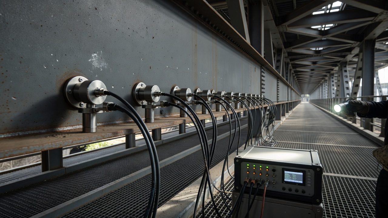
AE crack monitoring is implemented on in-service bridges, pressure vessels, and aerospace structures through continuous or periodic monitoring. During bridge load testing per ASTM E2983, AE sensors are clustered around known fatigue-sensitive details — welded stiffener-to-girder connections, cope holes, cover plate ends, diaphragm connections, and welded attachments. The monitoring process records AE activity as the structure is loaded to progressively higher levels.
Critical thresholds for crack AE monitoring include: crack initiation — first appearance of 55-70 dBAE events at a specific location, particularly when Felicity ratio drops below 0.95; active crack growth — sustained AE event rate above 10-50 hits per minute with amplitudes above 65 dBAE, especially during constant load holds; critical crack growth — event rate exceeding 100 hits per minute with amplitudes above 80 dBAE, indicating transition to unstable propagation. Chai et al. (2022) established warning thresholds for CrMoV steel: when cumulative AE count exceeds 100 at a source location and absolute energy exceeds 40 mV·ms, the crack has reached 50% of critical length. Below 50 cumulative counts and 20 mV·ms energy, crack growth remains in early stages.
AE detects active corrosion processes through multiple emission mechanisms. Past corrosion — stabilized pits, existing rust layers, passivated surfaces — produces no detectable AE. Only ongoing electrochemical activity involving physical material disruption generates stress waves. The primary corrosion mechanisms producing detectable AE include:
Active pitting corrosion generates 45-70 dBAE events as the passive film ruptures locally and metastable pits form, grow, and repassivate. Each film rupture event produces a short-duration (10-100 μs), broadband AE burst. Pit growth produces continuous low-level AE as dissolution products accumulate. Detection frequencies are 100-400 kHz. Pit initiation rates correlate with AE event rate — studies show 1-10 AE events per pit nucleation event.
Hydrogen bubble formation and collapse generates 35-55 dBAE signals during cathodic corrosion processes. Hydrogen bubbles nucleate on the corroding surface, grow through hydrogen gas accumulation, detach, and sometimes collapse — each phase producing characteristic AE. Bubble nucleation produces short 50-200 μs bursts. Bubble detachment produces longer 200-500 μs events. Detection frequencies are 100-300 kHz.
Stress corrosion cracking (SCC) generates 55-85+ dBAE emissions from both crack initiation (film rupture at crack tip) and crack propagation (micro-cleavage, intergranular separation). SCC emissions are characterized by high event rates during periods of active cracking, with frequent AE clusters (multiple hits within milliseconds from the same source). Detection frequencies are 100-500 kHz.
Crevice corrosion produces low-level continuous AE (ASL 30-55 dBAE) from ongoing dissolution within the crevice, with occasional higher amplitude events from localized film rupture. Uniform corrosion produces minimal detectable AE — the dissolution occurs over a large area, and the small-scale surface changes release insufficient strain energy for reliable detection.
| Corrosion Type | Amplitude (dBAE) | Frequency (kHz) | Duration (μs) | Distinguishing Features |
|---|---|---|---|---|
| Uniform corrosion | 30-45 | 100-300 | 50-200 | Continuous low-level, difficult to detect |
| Pitting corrosion | 45-70 | 100-400 | 10-100 | Discrete bursts, event rate = pit rate |
| Crevice corrosion | 35-55 | 100-300 | 50-500 | Continuous with occasional bursts |
| Stress corrosion cracking | 55-85+ | 100-500 | 100-1000+ | High event rate, frequent clusters |
| Hydrogen bubble | 35-55 | 100-300 | 50-500 | Three distinct phases (nucleation, growth, detachment) |
Jomdecha et al. (2007, Corrosion Science) characterized four corrosion types by amplitude distribution: uniform corrosion produced a narrow amplitude range of 30-45 dBAE, pitting produced a broader range of 45-70 dBAE with a characteristic bimodal distribution reflecting metastable (45-55 dBAE) and stable (55-70 dBAE) pit events, crevice corrosion showed 35-55 dBAE with a Gaussian distribution, and SCC showed 55-85+ dBAE with a positively skewed distribution.
Tendon wire breakage in prestressed or post-tensioned concrete bridges produces the highest energy AE events encountered in structural monitoring — typically 80-100+ dBAE with absolute energy levels 100-1000 times greater than typical crack propagation events. The wire break signature is characterized by: a single, extremely high amplitude transient with short rise time (<100 μs), long duration (1-20 ms including reflections), wide frequency content from 5-200 kHz, and a characteristic “ringing” decay as the released strain energy propagates multiple reflections along the tendon length.
The frequency content of tendon wire breaks peaks in the 20-80 kHz range — lower than most crack-related AE — due to waveguide effects in the tendon duct where the steel wire acts as a cylindrical waveguide. The released energy propagates primarily as guided longitudinal and flexural modes in the wire, with velocity around 4900-5100 m/s in sound grouted tendons and slightly lower (4700-4900 m/s) in ungrouted or partially grouted ducts.
AE sensor selection for wire break detection favors 60 kHz or 80 kHz resonant sensors (R6I or R80I models) positioned directly on anchor heads, at deviator saddles, or clamped to exposed tendon segments at intermediate locations. Sensor spacing for reliable wire break detection along a tendon duct is 1-5 m for embedded sensors in grouted ducts and up to 10 m for sensors on exposed anchor heads.
Wire break detection in operational bridges must discriminate true wire failure events from environmental and operational noise sources. A two-stage confirmation process is standard. Stage 1 — amplitude and energy threshold: events exceeding 90 dBAE with absolute energy above 10⁶ aJ are automatically flagged as potential wire breaks. Stage 2 — waveform analysis and multi-sensor correlation: the waveform is examined for characteristic wire break features including the presence of multiple wave modes (longitudinal and flexural), consistent frequency content across sensors, and arrival time patterns consistent with propagation along the tendon duct.
The Vallen DGZfP draft guideline for wire break detection specifies: minimum amplitude threshold of 80 dBAE, minimum signal strength threshold of 10⁶ pVs, and spatial consistency — the event must be detected on at least two sensors along the tendon axis. In the Altstädter Bahnhof (Halle, Germany) bridge monitoring case, 111 wire breaks were detected over 4 years of continuous monitoring, with 103 confirmed by subsequent visual inspection of extracted tendon sections. The three false positives were attributed to lightning strikes (2) and heavy construction equipment impact (1).
AE bridge load testing follows ASTM E2983 (Standard Guide for Application of Acoustic Emission to Structural Health Monitoring of Bridge Structures) and ISO 16837 (Non-destructive testing — Acoustic emission testing — Test method for damage qualification of reinforced concrete beams). These standards define sensor placement, loading protocol, data analysis criteria, and damage classification methodology.
The loading protocol per ASTM E2983 applies progressively increasing load steps, typically 20%, 40%, 60%, 80%, 90%, and 100% of the maximum test load with 5-minute holds at each step. During holds, AE activity should decay — sustained or increasing activity during a constant-load hold signals active damage. At 100% load, the structure is held for 10-30 minutes while monitoring AE activity. The final step may increase to 110-120% of the service load to evaluate the Kaiser effect on subsequent loading.
ISO 16837 damage classification uses the Load Ratio (L) — defined as the load at which AE resumes divided by the previous maximum load — and the Calm Ratio (C) — cumulative AE during unloading divided by total AE during the full cycle. These two parameters are plotted on a damage classification chart with three zones:
Low damage zone — Load Ratio > 0.9, Calm Ratio < 0.05. The structure shows strong Kaiser effect with minimal emissions during unloading. Damage is minor, and the structure is safe for continued service with routine monitoring.
Medium damage zone — Load Ratio 0.7-0.9, Calm Ratio 0.05-0.15. The Kaiser effect is partially violated, and unloading emissions indicate some structural instability. Detailed inspection is required to assess damage extent.
Severe damage zone — Load Ratio < 0.7, Calm Ratio > 0.15. The Kaiser effect is strongly violated, and high unloading activity indicates unstable conditions. Immediate intervention is required.
Tonelli et al. (2020, Sensors) demonstrated the application of this classification on a full-scale prestressed concrete bridge tested to failure, showing that the load ratio decreased progressively from 0.95 at low load levels to 0.45 at 80% of failure load, while the calm ratio increased from 0.02 to 0.32 over the same range.
The Cedar Avenue Bridge (Minnesota) monitoring project by TechKnowServ demonstrated a 16-sensor AE array on a steel tied-arch bridge. Sensors were deployed at 15 ft spacing along the floorbeam-to-girder connections identified as fatigue-prone details in the fracture control plan. Continuous monitoring over 18 months detected 237 active AE source locations, of which 22 were classified as crack growth events. Subsequent visual inspection and magnetic particle testing confirmed 19 cracks > 3 mm in length, with 16 at locations predicted by AE source clusters.
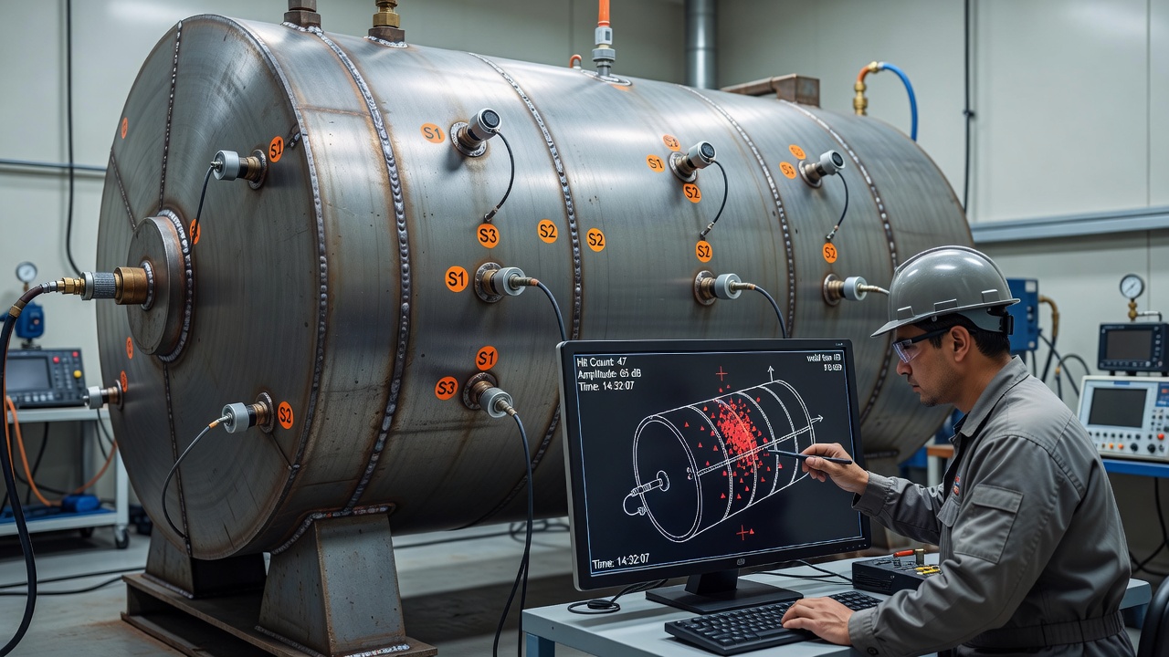
AE testing of pressure vessels and storage tanks is governed by multiple codes and standards. ASME Section V Article 12 covers AE examination of metallic pressure vessels during initial hydrotest and periodic requalification. ASME Section V Article 11 covers FRP equipment (tanks, pipes, vessels). ASME Section V Article 13 covers continuous AE monitoring of pressure vessels in service. ASTM E569 (Standard Practice for Acoustic Emission Monitoring of Structures During Controlled Stimulation) and ASTM E1930 (Standard Practice for Examination of Liquid-Filled Atmospheric and Low-Pressure Metal Storage Tanks Using Acoustic Emission) provide detailed procedures.
The standardized pressurization sequence for hydrotest per ASME guidelines proceeds in five steps: pressurize to 50% of test pressure and hold 5-10 minutes, record AE activity; increase to 65% and hold 10 minutes; increase to 85% and hold 10 minutes; increase to 100% of test pressure and hold 30 minutes; optionally increase to 110% (proof test level) for 5 minutes. During each hold period, the AE activity should decay following the Kaiser principle — a structure with no active damage shows rapidly decreasing hit rate during holds, while a damaged structure shows sustained or increasing activity.
AE sources detected during pressure vessel testing are graded by the activity (number of AE events per source) and intensity (average amplitude/energy of events): Grade A — minor, 1-10 hits, amplitude below 60 dBAE, considered insignificant; Grade B — mild, 10-50 hits, amplitude 60-75 dBAE, requires correlation with design stress analysis; Grade C — moderate, 50-200 hits, amplitude 75-85 dBAE, requires follow-up NDT (UT, radiography); Grade D — severe, 200-1000 hits, amplitude 85-95 dBAE, requires immediate evaluation and repair recommendation; Grade E — critical, >1000 hits, amplitude above 95 dBAE, requires shutdown and immediate repair before further pressurization.
Above-ground storage tank (AST) floor monitoring follows ASTM E1930 using the MONPAC system. A sensor array of 12-48 sensors (typically 60 kHz resonant) is deployed around the tank shell at 1-2 m spacing near the bottom. The tank is filled or the fill level varied while monitoring AE from floor corrosion, pitting, and leakage. Floor corrosion generates 45-75 dBAE events; active leakage through floor perforations generates continuous AE at 40-65 ASL dBAE. Source location accuracy in the floor plane is typically ±0.5-2 m depending on sensor spacing and liquid loading. API 653 (Tank Inspection, Repair, Alteration) recognizes AE as a screening method for tank floor condition, with AE results used to prioritize tanks for internal inspection and ultrasonic thickness gauging.
AE integrates with Structural Health Monitoring (SHM) systems through multi-sensor data fusion combining AE event data with strain measurements, accelerometer data, fiber optic sensors, environmental monitoring, and digital twin models. The integration architecture follows a layered approach.
The sensor layer combines AE sensors (20-100 per monitoring zone) with complementary sensing technologies: resistance strain gauges for local stress measurement, fiber Bragg grating (FBG) sensors for distributed strain and temperature, accelerometers for vibration-based global damage detection, and corrosion sensors (LPR, ER probes) for electrochemical monitoring. The data acquisition layer synchronizes AE hit data (microsecond timing) with slower parametric data (1-100 Hz sampling) through common time references — typically GPS time-stamped data acquisition systems.
The processing layer performs real-time source location, waveform classification, and noise filtering. Advanced systems use machine learning classifiers — support vector machines (SVM), k-nearest neighbors (k-NN), or neural networks — to classify AE sources into damage mechanism categories (crack, corrosion, wire break, fretting, noise). The diagnostics layer evaluates damage severity using Felicity ratio, AE event rate trends, amplitude distribution analysis, and b-value analysis (the slope of the amplitude-frequency distribution, where decreasing b-value indicates transition from microcracking to macrocracking).
The prognostics layer estimates remaining useful life by correlating AE intensity with fracture mechanics models. Cumulative AE energy is related to crack extension through Paris-law correlation, enabling estimation of crack growth rates and time to critical crack size. Digital twin integration maps AE source locations onto finite element model geometries, correlating AE activity with local stress intensity factors to predict damage progression under projected loading scenarios.

Wireless AE monitoring systems enable deployment on structures without hard-wired infrastructure. The MISTRAS Micro-SHM system provides 4-8 channels of AE monitoring in a compact, battery-powered enclosure with cellular or satellite backhaul. The Vallen WISAE (Wireless Smart AE) system supports distributed sensor nodes with local processing and wireless data transmission using 2.4 GHz or 868 MHz ISM band radios. Battery life for continuous monitoring ranges from 30 days (continuous streaming) to 2 years (periodic sampling with event-driven transmission). Solar-powered variants provide indefinite operation in remote locations including isolated bridge spans, pipeline pumping stations, and offshore platforms.
AE provides maximum value when integrated with complementary NDT methods for comprehensive structural assessment:
| NDT Method | Complementarity with AE | Integration Benefit |
|---|---|---|
| Ultrasonic Testing (UT) | UT sizes defects detected by AE; AE identifies active defects | AE finds active cracks, UT measures size and depth |
| Radiography (RT) | RT confirms internal defects detected by AE | AE screens large areas, RT verifies critical sources |
| Magnetic Particle (MT) | MT confirms surface crack indications from AE | AE detects subsurface crack growth before MT visibility |
| Eddy Current (ECT) | ECT characterizes surface defects near welds | AE locates active defects, ECT sizes and characterizes |
| Ground Penetrating Radar (GPR) | GPR locates rebar and ducts; AE detects active defects | GPR maps geometry, AE monitors structural integrity |
| Fiber Optic Sensing (FBG) | FBG measures strain; AE detects dynamic damage events | Strain state correlates with AE activity |
Real-time detection of active defects — AE detects damage as it occurs, providing immediate warning of crack initiation, propagation, and critical damage states. No other NDT method provides this temporal immediacy across an entire structure simultaneously.
Passive, non-invasive technique — AE does not inject energy into the structure, eliminating radiation hazards (RT), coupling requirements (UT), and equipment access needs (MT). Sensors mount on accessible surfaces without structural modification.
Global monitoring capability — A single AE sensor monitors a large area — up to 30 m radius in steel plate, 10-15 m in steel girder flanges, 3-5 m in concrete — enabling cost-effective monitoring of large structures from relatively few sensor locations.
Source location — AE provides spatial localization of damage sources, directing subsequent inspections to specific locations rather than requiring 100% coverage by other methods. Location accuracy of ±0.1-1 m in typical field deployments is sufficient to identify critical zones.
Continuous monitoring during service — AE operates during normal structural use — traffic loading on bridges, pressure cycling on vessels, thermal cycling on pipelines — capturing damage events that occur during operational conditions.
High sensitivity to early-stage damage — AE detects microcrack initiation at stress intensity factor ranges (ΔK) of 5-10 MPa√m in steel, well below the detection threshold of visual inspection (typically ΔK > 20-30 MPa√m for surface-breaking cracks) and ultrasonic testing (typically ΔK > 15-25 MPa√m).
Compatibility with automated systems — Modern AE systems provide automated event detection, source location, and alarm generation without requiring continuous operator attention. Thresholds and alert levels are programmable for unattended operation.
Fracture mechanics correlation — AE parameters — particularly cumulative counts and energy — correlate directly with crack extension through Paris law relationships, enabling quantitative damage assessment and remaining life estimation.
Applicability to multiple damage types — AE detects cracks, corrosion, wire breaks, delamination, fiber breakage, leaks, friction, impact, and yielding from a single sensor deployment with appropriate signal processing.
Proof test verification — AE during proof load tests immediately identifies active defect growth without requiring the structure to be loaded to failure, enabling safe qualification of pressure vessels, bridges, and aircraft structures.
Loading requirement — AE requires the structure to be stressed to generate emissions. A structure at rest with constant load and benign environmental conditions will produce no detectable AE regardless of damage state. This is the single most important operational limitation.
No defect sizing — AE detects defect activity but does not directly measure defect size. A large, active emission source may represent either a large crack growing rapidly or a small crack emitting intensely. Correlation between AE activity and defect size requires fracture mechanics models or complementary NDT.
Signal attenuation — AE signals attenuate with propagation distance due to geometric spreading, material absorption, and scattering. Sensor spacing must account for attenuation rates: steel plates 1 dB/m, concrete 3-8 dB/m, composites 10-30 dB/m, and interface-dominated structures (grouted tendons, layered composites) up to 50 dB/m.
Noise discrimination — Operational environments generate noise sources that can mask or be mistaken for AE signals: electromagnetic interference, mechanical vibration, rain impact, wind-induced movement, traffic rumble, hydraulic systems, and thermal expansion cracking. Noise filtering requires careful setup and often post-processing analysis.
Permanent sensor installation — Continuous monitoring requires sensors to remain mounted on the structure for the monitoring duration. Sensor installation, cable routing, and protection require engineering design and can be cost-prohibitive for short-term monitoring.
Coupling degradation — Over extended monitoring periods (months to years), sensor couplant degrades, adhesive bonds weaken, and magnetic clamps may shift. Periodic pencil-lead break verification per ASTM E976 is essential to maintain data quality.
Interpretation expertise — AE data interpretation requires understanding of material behavior, wave propagation, signal processing, structural mechanics, and damage mechanisms. Automated classification systems reduce but do not eliminate the need for experienced analysts.
No detection of dormant defects — AE detects only active or growing defects. Pre-existing damage that is stable and not growing under current conditions — a stabilized crack, a passivated corrosion pit, a previously yielded zone — produces no AE until it reactivates.
Cumulative AE calibration — The relationship between cumulative AE activity and structural degradation is material-specific, geometry-dependent, and loading-dependent. Calibration requires representative laboratory testing or field validation that may not exist for specific structures.
Environmental sensitivity — Temperature extremes affect sensor sensitivity (PZT properties shift above 150°C), couplant viscosity (grease hardens below -20°C), and cable electrical properties. High humidity corrodes sensor contacts. Lightning and power surges can damage sensitive preamplifiers.
| Standard | Title | Application |
|---|---|---|
| ASTM E1316 | Standard Terminology for NDT | AE definitions and terminology |
| ASTM E569 | AE Monitoring During Controlled Stimulation | In-service pressure vessel monitoring |
| ASTM E650 | Mounting Piezoelectric AE Sensors | Sensor installation procedures |
| ASTM E750 | AE Instrumentation Characterization | Data acquisition specifications |
| ASTM E976 | AE Sensor Response Characterization | Pencil-lead break calibration guide |
| ASTM E1067 | AE Examination of FRP Tanks/Vessels | Composite equipment monitoring |
| ASTM E1106 | Primary Calibration of AE Sensors | Metrological sensor calibration |
| ASTM E1419 | AE Examination of Seamless Gas Cylinders | Gas cylinder hydrotest monitoring |
| ASTM E1781 | Secondary Calibration of AE Sensors | Field sensor verification |
| ASTM E1930 | AE Examination of Atmospheric Storage Tanks | Tank floor corrosion monitoring |
| ASTM E2075 | AE Sensor Response from Simulated AE | Hsu-Nielsen source standard |
| ASTM E2374 | AE Examination of Composite Structures | Composite structural monitoring |
| ASTM E2983 | AE for SHM of Bridges | Bridge monitoring procedures |
| ISO 16837 | AE for Damage Qualification of RC Beams | Concrete bridge damage classification |
| ISO 16838 | AE for Integrity Assessment | Structural integrity protocol |
| ASME V Art. 11 | AE Examination of FRP Equipment | FRP tank/vessel testing |
| ASME V Art. 12 | AE Examination of Metallic Vessels | Metal vessel hydrotesting |
| ASME V Art. 13 | Continuous AE Monitoring | In-service continuous monitoring |
| EN 1330-9 | AE Terminology | European terminology standard |
| EN 13477-1/2 | AE Equipment Characterization | European equipment standard |
| EN 13554 | AE General Principles | European general principles |
| EN 14584 | AE Testing of Metallic Pressure Equipment | European pressure equipment standard |
| EN 15495 | AE Zonal Location | European zonal location method |
| EN 15856 | AE for Corrosion Detection | Corrosion monitoring standard |
| EN 15857 | AE for Fiber-Reinforced Polymers | FRP monitoring standard |
TarmacView structural health monitoring platform supports integration with continuous AE monitoring systems — combining real-time stress wave detection with AI-powered defect classification, source location visualization, and digital twin correlation for bridges, tunnels, and airfield pavements.
Impact-Echo is a stress-wave nondestructive testing method where a short-duration mechanical impact on a concrete surface generates stress waves that reflect fr...
Ultrasonic Testing (UT) uses high-frequency sound waves (typically 20 kHz–200 MHz) to detect internal flaws, measure thickness, and assess material properties i...
Non-Destructive Testing (NDT) encompasses methods to evaluate material properties, detect defects, and assess structural condition without causing damage. For i...