Crack Segmentation
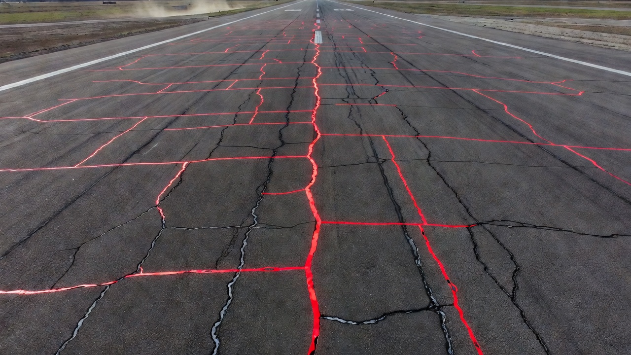
Crack segmentation is the computer vision task of classifying every pixel in an image as either crack or non-crack, producing a binary mask that enables precise...
32 min read
Computer Vision
Deep Learning
+2
AI-based crack detection uses computer vision — convolutional neural networks, vision transformers, and semantic segmentation models — to automatically identify, classify, and measure cracks in pavement and structural imagery. The technology underpins automated road, runway, and bridge inspection programs across the civil aviation and transportation sectors.
AI-based crack detection is a computer vision technology that applies deep learning models — convolutional neural networks (CNNs), encoder-decoder architectures, and vision transformers — to automatically identify, classify, segment, and measure cracks in pavement, runway, bridge deck, and concrete structural surfaces from digital imagery. The technology replaces or augments manual visual inspection by human engineers, transforming subjective, labor-intensive surveys into objective, scalable, data-driven assessments. For airport and civil infrastructure operators, automated crack detection directly supports Pavement Condition Index (PCI) scoring per ASTM D5340-12, Runway Condition Code (RwyCC) reporting per ICAO Annex 14, and preventive maintenance planning.
The crack detection problem presents unique challenges that distinguish it from general semantic segmentation tasks. Cracks are thin, elongated structures — typically 0.1 mm to 5 mm in width — that occupy only 2–8% of total pixels in any given image, creating extreme class imbalance during model training. The foreground-to-background ratio for crack pixels is approximately 1:20 to 1:50, meaning a naive classifier that predicts all pixels as background achieves 95%+ accuracy while detecting zero cracks. Crack morphology varies dramatically: longitudinal cracks run parallel to the pavement centerline, transverse cracks run perpendicular, alligator (fatigue) cracks form interconnected polygonal patterns, and reflection cracks propagate through overlays from underlying joints. Each type requires different geometric characterization.
Illumination and environmental variability further complicate detection. Shadows from structures and overhanging vegetation create low-contrast regions where cracks become nearly invisible. Wet pavement reduces surface temperature contrast for thermal-based methods and alters visible-spectrum reflectivity. Oil stains, tire marks, rubber deposits, construction joints, surface texture variations (tining, grooving, broom finish), and debris produce false-positive features that visually mimic cracks. A 2025 study published in Scientific Reports (EGA-UNet paper, Vol. 15, Article 33818) demonstrated that crack detection accuracy on complex backgrounds degrades by 10–20% compared to clean, uniform surfaces, even with state-of-the-art attention mechanisms.
Scale and resolution constraints impose a fundamental trade-off. High-resolution imagery (sub-millimeter per pixel ground sampling distance) captures fine cracks but requires large storage, bandwidth, and processing time. Lower-resolution imagery covers more area per flight or drive but misses cracks narrower than 2–3 pixels. For drone-based runway inspection at 15 m altitude with a 24 MP camera, typical ground sampling distance is 1.0–1.5 mm/pixel, meaning cracks below 0.3 mm width fall below the detection threshold. This resolution limit is a hard physical constraint that no AI model can overcome — it governs the minimum detectable crack width for any given imaging platform and altitude.
U-Net, introduced by Ronneberger, Fischer, and Brox at the University of Freiburg in 2015, remains the most widely adopted architecture for pixel-level crack segmentation. The architecture’s symmetric encoder-decoder structure with skip connections is particularly well-suited for crack detection because cracks are thin, spatially localized features that require preservation of high-frequency detail throughout the downsampling and upsampling pipeline.
The U-Net encoder (contracting path) consists of four downsampling blocks. Each block contains two 3×3 convolutions (padding=same) followed by ReLU activation and a 2×2 max pooling operation (stride=2). The filter count doubles at each level: 64 → 128 → 256 → 512 → 1024 at the bottleneck. For a 512×512 pixel input, the spatial dimensions reduce through the encoder as 512 → 256 → 128 → 64 → 32 at the deepest layer. The bottleneck layer at the bottom of the U-shape contains 1024 feature maps at 32×32 resolution, representing the most abstract, semantically rich features.
The decoder (expanding path) mirrors the encoder with four upsampling blocks. Each block applies a 2×2 transposed convolution (deconvolution) that halves the number of filters and doubles the spatial dimensions. The upsampled feature map is concatenated with the corresponding feature map from the encoder path via skip connections — for example, the decoder’s 128×128 layer receives a direct concatenation from the encoder’s 128×128 layer. This skip connection mechanism is critical: it provides the decoder with high-resolution spatial details from the encoder that would otherwise be lost during the aggressive downsampling. After concatenation, two 3×3 convolutions with ReLU refine the combined features.
The final output layer is a 1×1 convolution with sigmoid activation, producing a single-channel probability map where each pixel value (0 to 1) represents the probability of that pixel belonging to a crack region. A threshold (typically 0.5) converts probabilities to binary crack/non-crack segmentation.
The original U-Net contains ~31 million parameters and 23 convolutional layers. For a 512×512 input, inference speed is approximately 40 ms per image on a modern GPU (NVIDIA RTX 3080 or equivalent). Lightweight variants such as ResU-Net (using residual connections instead of plain convolutions) reduce parameters to ~7.8 million while achieving 68.47% mean IoU on crack datasets. EGA-UNet further reduces to ~2.3 million parameters while improving Dice to 73.1% through ghost convolutions and Fourier-based token mixing.
U-Net’s skip connections are architecturally essential for crack detection. Without them, thin cracks (1–5 pixels wide) would be completely lost during the 4× downsampling (32× reduction at bottleneck) — a 3-pixel-wide crack at the input becomes a sub-pixel feature at the bottleneck that cannot be recovered by upsampling alone. The skip connections bypass this information bottleneck entirely, providing the decoder with the full-resolution crack geometry from the encoder.
DeepLabV3+, developed by Chen et al. at Google in 2018, addresses crack detection through atrous (dilated) convolutions and the Atrous Spatial Pyramid Pooling (ASPP) module. Unlike U-Net, which aggressively downsamples and recovers via skip connections, DeepLab maintains higher-resolution feature maps throughout the backbone by using dilated convolutions that expand the receptive field without reducing spatial dimensions.
The backbone is typically ResNet-101 (101 layers, ~42.6 million parameters) or Xception-65 (~54.7 million parameters). Standard convolutions in the backbone are replaced with atrous convolutions — 3×3 kernels with dilation rates (holes) inserted between kernel elements. A 3×3 kernel with dilation rate r=2 covers a 5×5 receptive field; r=4 covers 9×9; r=8 covers 17×17; and r=16 covers 33×33 — all with the same parameter count (9 weights) as a standard 3×3 convolution. This property is critical for crack detection: it enables the model to see larger context around each pixel (distinguishing cracks from surface texture) without the resolution loss that would occur from downsampling.
The ASPP module applies four parallel atrous convolutional branches with dilation rates r=6, 12, 18, and 24 (for output stride=16), each with 256 filters and 3×3 kernels. An additional 1×1 convolution branch and an image-level pooling branch (global average pooling → 1×1 convolution → bilinear upsampling) complete the module. All five branches produce 256-channel feature maps that are concatenated and passed through another 1×1 convolution. The ASPP module’s multi-scale capability is particularly important for cracks that vary significantly in width — a hairline crack (<1 mm) and a wide crack (>6 mm) require different receptive field sizes for optimal detection.
The DeepLabV3+ decoder is lightweight compared to U-Net’s full decoder: bilinear upsampling by 4×, concatenation with low-level features from an early backbone layer (reduced to 48 channels via 1×1 convolution), two 3×3 convolutions (256 filters), and final bilinear upsampling by 4× to the original resolution. The output stride is typically 16 (input resolution divided by 16 at bottleneck), sometimes 8 for denser feature maps at the cost of 2× memory usage.
DeepLabV3+ achieves approximately 78.5% mIoU on crack datasets. However, the EGA-UNet study (2025) reported that DeepLabV3+ underperforms lightweight architectures like EGA-UNet (73.1% Dice vs. lower for DeepLabV3+) due to insufficient fine detail preservation at crack boundaries. The ASPP module’s dilations, while effective for multi-scale context, blur fine spatial details that are essential for accurate crack width measurement.
Vision Transformers (ViT) , introduced by Dosovitskiy et al. at Google in 2020, apply the Transformer self-attention architecture — originally developed for natural language processing — to image analysis. ViT divides an input image into non-overlapping patches of size P×P (typically 16×16 pixels), linearizes each patch into a vector, and processes the sequence of patch embeddings through standard Transformer encoder layers with multi-head self-attention.
For a 224×224 input with 16×16 patches, ViT produces (224/16)² = 196 patch embeddings. Each patch of dimensions 16×16×3 (RGB) is flattened to a 768-dimensional vector and linearly projected to the embedding dimension D. The Transformer encoder consists of L stacked layers. ViT-Base uses L=12, D=768, and 12 attention heads (86M parameters). ViT-Large uses L=24, D=1024, and 16 heads (307M parameters). ViT-Huge uses L=32, D=1280, and 16 heads (632M parameters). Self-attention complexity scales as O(n²·D) where n is the number of patches — 196 patches with D=768 requires approximately 28 million operations per head per layer.
For crack segmentation, ViT is used as a backbone in hybrid encoder-decoder architectures. TransUNet replaces the U-Net encoder with a ViT, combining Transformer global context with a CNN decoder for fine detail recovery. SwinUNet uses a hierarchical Swin Transformer with shifted windows to reduce the O(n²) computational cost. SETR (SEgmentation TRansformer) applies ViT directly as an encoder with progressive upsampling.
The advantage of ViT for crack detection lies in its global receptive field. CNNs process information locally, requiring many layers to propagate information across large spatial distances. ViT’s self-attention mechanism connects every patch to every other patch in a single layer, enabling it to detect long, continuous cracks that span hundreds or thousands of pixels — fatigue cracks that meander across an entire runway width, for instance. Hybrid ViT-CNN models achieve 74–78% IoU on crack datasets, with TransUNet showing particular strength on alligator (interconnected) crack patterns.
The critical limitation is computational cost. A 512×512 image divided into 16×16 patches produces (512/16)² = 1,024 patches, requiring 1,024² ≈ 1 million attention computations per layer — an order of magnitude more than 196 patches for 224×224 inputs. This makes full ViT deployment on edge devices (drones, mobile inspection vehicles) impractical without significant compression or pruning.
DINOv3, released by Meta AI in 2025, represents the state of the art in self-supervised Vision Transformers. It is the third generation of the DINO (DIstillation with NO labels) family, trained at unprecedented scale: up to 7 billion parameters on 1.7 billion unlabeled images. DINOv3 uses a teacher-student framework where the student learns to match the teacher’s output representations without any human-labeled data.
The key architectural innovation in DINOv3 is Gram Anchoring — a regularization technique applied after approximately 1 million training iterations that stabilizes dense (patch-level) feature representations. The student model’s Gram matrix (pairwise patch similarity, dimensions N×N where N=number of patches) is constrained to remain close to a frozen “Gram teacher” copy. This prevents dense feature collapse, a failure mode in self-supervised learning where distinct image patches converge to similar embeddings despite being semantically different. Earlier DINO variants (v1 and v2) suffered from this collapse during extended training; Gram Anchoring enables stable training across billions of images.
For crack detection, DINOv3’s relevance lies in the frozen backbone paradigm. The pretrained ViT backbone (available in sizes from ViT-Small at 21M parameters to ViT-Huge at 632M and the flagship 7B model) is frozen and used as a universal visual encoder. Lightweight task-specific heads — linear probes, MLP adapters, or small convolutional heads — are trained on top without backpropagating through the backbone. This enables:
DINOv3’s patch-level features (rather than global image embeddings) preserve fine-grained spatial information needed for thin crack delineation. The ViT-Base variant (86M parameters, 12 layers, 768 embedding dimension) provides the best accuracy-to-compute ratio for infrastructure inspection applications. DINOv3 is particularly promising for runway inspection programs where labeled crack data is scarce — a common scenario for smaller airports without extensive pavement management history.
CrackNet, developed by Zhang et al. in 2017 at the University of South Florida, was one of the first deep CNN architectures designed specifically and exclusively for automated pavement crack detection. Unlike general-purpose architectures (U-Net, DeepLab) adapted from biomedical or natural image segmentation, CrackNet was architected from the ground up for pavement crack morphology.
The original CrackNet architecture consists of 6 convolutional layers with a fully connected top: Conv1 (5×5, stride=1, 64 filters) → Conv2 (5×5, stride=1, 64 filters) → MaxPool (2×2) → Conv3 (3×3, stride=1, 128 filters) → Conv4 (3×3, stride=1, 128 filters) → MaxPool (2×2) → Conv5 (5×5, stride=1, 256 filters) → Conv6 (3×3, stride=1, 256 filters) → Fully Connected (2,048 units) → Softmax output (2 classes: crack or non-crack). Total parameter count is ~1.4 million — approximately 22× smaller than U-Net (31M) and 35× smaller than DeepLabV3+ (42–55M).
CrackNet operates on fixed-size 64×64 pixel patches rather than full images. The training dataset comprised 640,000 patches extracted from 1,800 pavement images (160,000 for validation, 180,000 for testing). Each patch is classified as containing a crack in the center pixel or not — this is a patch-based classification approach rather than pixel-level segmentation. Modern variants (CrackNet-V, CrackNet-II, CrackNet-R) replaced the patch classifier with fully convolutional networks for dense pixel-level prediction.
CrackNet-V (the 2020 improved variant) added Generative Adversarial Network (GAN)-based training. The generator produces crack segmentation maps from input images, and a discriminator network distinguishes generated maps from ground truth annotations. This adversarial training regime improved F1-score to 0.87 on the CFD dataset. CrackNet-V also introduced multi-scale feature fusion with inception-style modules, enabling detection of cracks at varying widths.
CrackNet’s significance is architectural efficiency for edge deployment. At 1.4M parameters and 5 ms per patch, it demonstrated that crack-specific architecture design could achieve production-grade accuracy on the hardware available in 2017 — a single NVIDIA Tesla K80 GPU could process a full pavement image (stitched from patches) in under 2 seconds. This established the feasibility of real-time automated crack detection for highway-speed survey vehicles.
EGA-UNet, published by Yang et al. in Scientific Reports (Vol. 15, Article 33818, 2025), represents the current state-of-the-art for efficient crack segmentation. The architecture achieves 73.1% Dice coefficient with only ~2.3 million parameters — approximately 13× smaller than standard U-Net while improving accuracy by +3.1% Dice over U-Net, +11.9% over SegNet, and +44.9% over PSPNet on benchmark crack datasets.
Three architectural innovations distinguish EGA-UNet:
EG-Block (Efficient Ghost Sparse Convolution Block): This building block uses “ghost” convolution — a technique that generates a small number of intrinsic feature maps via standard convolution and then applies cheaper linear operations (3×3 depthwise convolutions) to produce additional “ghost” feature maps. For a desired output of C channels, ghost convolution generates approximately C/2 via standard conv and C/2 via linear operations, reducing computation by approximately 50% compared to standard convolution at equivalent output channels. The EG-Block incorporates an Efficient Multi-scale Attention (EMA) module that weights features across multiple spatial scales.
A-RepViT Block: This replaces the standard Vision Transformer token mixer with Adaptive Fourier Filtering (AFF) . The input feature map is transformed to the frequency domain via Fast Fourier Transform (FFT), frequency components are adaptively filtered (low-pass, high-pass, or band-pass depending on learned weights), and the inverse FFT reconstructs the spatial feature map. AFF captures global context with O(n log n) complexity versus O(n²) for self-attention — for a 32×32 feature map (1,024 elements), this reduces computation from ~1M operations to ~10K operations per layer.
SPPF (Spatial Pyramid Pooling Fast): Applied in the deepest encoder layer, SPPF aggregates multi-scale features using three sequential max-pooling operations of varying kernel sizes (5×5, 9×9, 13×13 effective receptive fields), concatenated into a unified multi-scale representation. This is computationally efficient compared to parallel ASPP (used in DeepLab) because the sequential pooling reuses intermediate results.
EGA-UNet’s inference speed is sufficient for real-time edge deployment. On an NVIDIA Jetson Orin Nano Super, the model achieves approximately 45–55 FPS at FP16 precision on 512×512 inputs, making it suitable for drone-based or vehicle-mounted real-time crack detection. The lightweight design enables deployment on platforms without dedicated GPUs — inference at 8–12 FPS on a Raspberry Pi 5 with Hailo-8L NPU accelerator (13 TOPS) has been demonstrated.
| Architecture | Parameters | Design Principle | Key Innovation | Crack Dice/IoU | Edge-Deployable |
|---|---|---|---|---|---|
| U-Net (2015) | ~31M | Encoder-decoder, skip connections | Spatial detail preservation | 65–68% IoU | With quantization |
| ResU-Net | ~7.8M | Residual skip connections | Gradient flow improvement | 68.5% IoU | Yes |
| DeepLabV3+ (2018) | ~42–55M | Atrous convolution, ASPP | Multi-scale context | ~75% IoU | No |
| ViT-Base (2020) | 86M | Self-attention on patches | Global receptive field | 74–78% IoU | No |
| DINOv3 (2025) | 21M–7B | Self-supervised, frozen backbone | Few-shot transfer | Comparable supervised | With adapter head |
| CrackNet (2017) | ~1.4M | Patch-based CNN | Pavement-specific design | ~87% F1 (patch) | Yes |
| EGA-UNet (2025) | ~2.3M | Ghost conv + AFF token mixing | Lightweight + global context | 73.1% Dice | Yes |
Training crack detection models requires pixel-level annotated datasets where each image has a corresponding binary mask labeling every pixel as crack (white, value 1) or non-crack (black, value 0). The annotation process is labor-intensive — a single 2000×1500 pixel image requires 15–45 minutes of expert manual labeling using polyline drawing tools followed by morphological dilation to produce full-width crack masks. The following datasets constitute the standard benchmarks for academic research and model development.
Crack500, published by Yang et al. in 2020, contains 500 RGB images at 2000×1500 pixel resolution (3 megapixels per image). Images were captured using mobile phone cameras on pavement surfaces around Temple University in Philadelphia, USA. Each image has a corresponding pixel-level binary segmentation mask annotated manually using polyline drawing tools. Researchers commonly subdivide the 500 images into approximately 1,896 non-overlapping 512×512 patches for model training. The standard split allocates 350 images for training, 50 for validation, and 100 for testing. Crack pixels constitute approximately 2–5% of total pixels per image. Crack widths range from 0.1 mm to 5 mm, and images include multiple lighting conditions (sunny, overcast, shadowed). Crack types include longitudinal, transverse, and alligator patterns.
DeepCrack, published by Liu et al. in Neurocomputing (2019), contains 537 RGB images at 544×384 pixel resolution. Images were captured from diverse concrete and asphalt surfaces — bridges, roads, tunnels, and building walls — providing multi-scene coverage uncommon in single-source pavement datasets. Each image has pixel-level binary annotations as PNG masks. The dataset is pre-split into approximately 300 training and 237 test images. DeepCrack was specifically built to evaluate the Holistically-Nested Edge Detection (HED) architecture adapted for crack detection. The dataset includes challenging conditions: low contrast between cracks and background, thin cracks (1–3 pixels wide), and textured surface backgrounds. Cracks are categorized by width rather than structural type.
CFD, published by Shi et al. in IEEE Transactions on Intelligent Transportation Systems (2016), contains 118 images at 480×320 pixel resolution. Images were captured using an iPhone 5 on urban roads in Beijing, China. Each image has pixel-level manual ground truth masks, plus a “seg” folder with superpixel-based segmentations. The dataset was designed to reflect general urban road surface conditions and includes noise factors: shadows from trees and buildings, oil stains, water puddles, and leaf coverage. Crack pixels account for approximately 4–8% of each image. The low 480×320 resolution makes thin crack detection challenging — cracks can be as narrow as 1–2 pixels. CFD is licensed for non-commercial research use only with citation requirement. Its primary limitation is small size (118 images), single geographic area, and single camera.
GAPs384 (German Asphalt Pavement Distress dataset) , from Ilmenau University of Technology, Germany, contains 1,969 images at 1920×1080 pixel resolution (Full HD). This is the largest single-source public crack dataset by image count. Images are grayscale (not RGB), which reduces file size but eliminates color information that can aid crack discrimination. Annotations include crack type classification (longitudinal, transverse, alligator) in addition to pixel-level crack masks. The high resolution and consistent capture conditions (German highway network) make GAPs384 valuable for training models intended for European pavement conditions. The dataset includes a wider range of crack severities than CFD or Crack500.
NHA12D, published by Huang et al. (2022), contains 80 pavement images collected from the UK A12 highway network by National Highways (formerly Highways England). The dataset uniquely includes 40 concrete pavement images and 40 asphalt pavement images captured under identical survey conditions by digital survey vehicles. This dual-surface composition makes NHA12D valuable for evaluating cross-domain generalization — a model’s ability to detect cracks on both surface types without degradation. Pixel-level ground truth annotations are provided. The small size (80 images) makes NHA12D primarily a benchmark dataset rather than a training resource.
| Dataset | Images | Resolution | Crack %/Image | Source | Year |
|---|---|---|---|---|---|
| Crack500 | 500 | 2,000×1,500 | 2–5% | Philadelphia roads | 2020 |
| DeepCrack | 537 | 544×384 | varies | Multi-scene | 2019 |
| CFD | 118 | 480×320 | 4–8% | Beijing roads | 2016 |
| GAPs384 | 1,969 | 1,920×1,080 | varies | German highways | 2020 |
| NHA12D | 80 | High-res | varies | UK A12 highway | 2022 |
| CrackTree200 | 206 | 800×600 | varies | Pavement (challenging) | 2012 |
All crack datasets exhibit severe class imbalance: crack pixels constitute 2–8% of total pixels, meaning models must learn from an average of 500–2,000 crack pixels per 25,000-total-pixel image (480×320 CFD resolution). Standard cross-entropy loss is ineffective — a model minimizes loss by predicting “background” for every pixel. Specialized loss functions address this:
Focal Loss (Lin et al., 2017) applies a modulating factor (1 − pt)γ to the cross-entropy loss, where pt is the model’s predicted probability for the ground-truth class and γ is a focusing parameter (typically 2.0). This down-weights well-classified examples (pt → 1.0) and up-weights hard, misclassified examples (pt → 0.0). For crack detection with γ=2.0, focal loss reduces the contribution of easy background pixels by approximately 4× compared to cross-entropy.
Dice Loss (Milletari et al., 2016) = 1 − Dice coefficient = 1 − (2TP + ε)/(2TP + FP + FN + ε). This directly optimizes the evaluation metric. Dice loss is less sensitive to class imbalance than cross-entropy because it measures overlap rather than per-pixel accuracy. It is the standard loss function for U-Net-based crack segmentation.
Tversky Loss (Salehi et al., 2017) generalizes Dice loss by weighting false positives and false negatives differently: Tversky index = TP/(TP + α·FP + β·FN). For safety-critical crack detection where false negatives (missed cracks) are more dangerous than false positives (false alarms), setting α=0.3 and β=0.7 penalizes FN more heavily than FP.
SupContrast (Supervised Contrastive Loss) , relevant to DINOv3-based approaches, pulls patch embeddings of crack pixels together in embedding space while pushing them apart from background pixel embeddings. This creates a well-structured embedding space where crack pixels form tight clusters that are linearly separable from background clusters.
AI-based crack detection approaches fall into two methodological categories: classification-based and segmentation-based, each with distinct outputs, metrics, and use cases.
Crack classification determines whether an image region (image patch, tile, or full image) contains a crack. The output is a binary label (crack present / crack absent) or a multi-class label (crack type: longitudinal, transverse, alligator). Classification models are typically lightweight CNNs (CrackNet at 1.4M parameters, MobileNetV2 at 3.5M parameters) trained on patch-level datasets. The output provides crack presence probability and location (which patch contains a crack) but does not provide crack geometry — width, length, orientation, or topology. Classification is appropriate for rapid screening surveys where the goal is to identify crack locations for follow-up inspection, not to measure individual cracks. Evaluation uses accuracy, precision, recall, and F1 at the patch or image level.
Crack segmentation (semantic segmentation) classifies each pixel individually as crack or non-crack. The output is a binary mask at the same resolution as the input image, where every pixel has a crack probability. This provides full crack geometry — width at every point along the crack, total length, orientation angle, branching topology, and crack area. Segmentation is required for quantitative pavement condition assessment (PCI calculation, crack width severity classification per ICAO standards). Evaluation uses pixel-level metrics: IoU, Dice, precision, recall, and boundary F1. Segmentation models are computationally heavier (U-Net at 31M parameters, DeepLabV3+ at 42–55M) but provide substantially richer output.
Some systems use instance segmentation (detecting each individual crack as a separate object), which distinguishes between disconnected cracks. This is relevant for crack counting (number of cracks per unit area) and crack density mapping. Mask R-CNN and YOLOv8-seg are common instance segmentation architectures for crack detection.
IoU (Jaccard Index) measures the overlap between predicted crack segmentation and ground truth, divided by the union of both. It is the most widely reported metric for crack segmentation:
IoU = TP / (TP + FP + FN)
Values range from 0 (no overlap) to 1 (perfect overlap). Typical IoU for crack detection models ranges from 0.55 to 0.75. IoU is more sensitive than Dice to false positives and false negatives because the union denominator is larger than the individual sums. A model predicting a 100-pixel ground truth crack with 60 correct pixels (TP=60, FP=20, FN=40) achieves IoU = 60/(60+20+40) = 0.50. The stricter union denominator means IoU is always lower than or equal to Dice for the same prediction.
Dice (also called F1 score for binary segmentation) is the harmonic mean of precision and recall:
Dice = 2 × TP / (2 × TP + FP + FN)
Dice relates to IoU: Dice = 2·IoU / (1 + IoU). For the example above (IoU=0.50), Dice = 2×0.50/1.50 = 0.67. Typical Dice for crack detection ranges from 0.65 to 0.80. The EGA-UNet paper (2025) reports Dice = 73.1% as their primary metric. Dice gives a more optimistic assessment of segmentation quality than IoU, and the gap between the two widens as quality decreases — a low-quality prediction with IoU=0.25 has Dice=0.40.
Precision (Positive Predictive Value) = TP/(TP+FP). Measures false alarm rate: of all pixels labeled crack, what fraction is actually crack? High precision (>0.85) means few false positives. Important when crack detection triggers costly follow-up actions (e.g., sealing crews dispatched to inspect flagged locations).
Recall (Sensitivity, True Positive Rate) = TP/(TP+FN). Measures missed crack rate: of all actual crack pixels, what fraction did the model detect? High recall (>0.85) means few missed cracks. For safety-critical infrastructure (runway inspection at commercial airports), recall is prioritized over precision — investigating a false alarm is less consequential than missing a real crack that could propagate into a structural failure under aircraft loading.
mAP evaluates precision across different recall thresholds, typically reported at IoU thresholds of 0.50 (mAP@50) and from 0.50 to 0.95 in 0.05 increments (mAP@50:95). For crack detection as an object detection task (bounding boxes), mAP measures how well the model localizes crack regions. A 2025 University of Central Florida study using Grounding DINO for thermal crack detection achieved 70% mAP@[0.5:0.95]. For pixel-level segmentation tasks, IoU and Dice are preferred over mAP because cracks are non-rectangular structures and bounding box metrics poorly represent segmentation quality.
| Metric | Formula | Range | Typical Crack Value | Use Case |
|---|---|---|---|---|
| IoU | TP/(TP+FP+FN) | 0–1 | 0.55–0.75 | Segmentation quality (strict) |
| Dice | 2TP/(2TP+FP+FN) | 0–1 | 0.65–0.80 | Segmentation quality (lenient) |
| Precision | TP/(TP+FP) | 0–1 | 0.80–0.95 | False alarm control |
| Recall | TP/(TP+FN) | 0–1 | 0.80–0.95 | Safety-critical detection |
| F1 | 2PR/(P+R) | 0–1 | 0.80–0.92 | Overall |
| mAP@50 | Avg precision at IoU≥0.5 | 0–1 | 0.70–0.85 | Object detection |
| Pixel Accuracy | (TP+TN)/(TP+TN+FP+FN) | 0–1 | >0.95 (misleading) | Not recommended for cracks |
The binary segmentation mask output from an AI model provides crack location and shape, but infrastructure inspection standards require physical crack dimensions — width in millimeters, length in meters, and area in square millimeters. Converting pixel-level masks to engineering measurements requires a computational geometry pipeline.
Skeletonization (thinning) reduces the crack region to a single-pixel-wide centerline that preserves crack topology (connectivity, branching, endpoints). The Zhang-Suen thinning algorithm (1984) is the standard method:
The Medial Axis Transform (MAT) is an alternative using the distance transform: for each interior crack pixel, compute the minimum Euclidean distance to the crack boundary. The skeleton consists of pixels that are local maxima in this distance map. MAT produces smoother skeletons for thick, irregular cracks but requires O(n²) computation versus O(n) for Zhang-Suen thinning.
The Euclidean Distance Transform (EDT) calculates the minimum Euclidean distance from each skeleton pixel (x,y) to the nearest crack boundary pixel:
D(x,y) = min(i,j)∈∂C √((x−i)² + (y−j)²)
where ∂C is the set of boundary pixels of the crack region. Crack width at point (x,y) = 2 × D(x,y), because the distance from the centerline to the boundary is half the full crack width.
The distance transform is computed efficiently using:
cv2.distanceTransform(): O(n) two-pass raster scan producing approximate Euclidean distance with <1% errorWidth statistics derived from the per-pixel width array:
Crack length is measured from the skeletonized centerline:
Method 1 — Pixel Counting with Connectivity Correction:
Method 2 — Chain Code (Freeman Chain):
Method 3 — Euclidean Distance Between Ordered Points:
For branching cracks (e.g., alligator cracking near intersections), the total crack length includes all branches. The skeleton must be decomposed into individual branches at junction points before length calculation.
Segmentation masks measure cracks in pixels; engineering standards require physical millimeters. Four calibration methods are used:
1. Known Reference Object: Place an object of known dimensions (coin, ruler, or calibration target) in the scene. Scale factor S = known_length_mm / measured_length_pixels. Accuracy: ±0.5–1%.
2. Laser Projection (Carrasco et al., 2021): Two parallel laser beams at known distance (e.g., 50 mm) are projected onto the surface. The pixel distance between laser spots gives S = 50 mm / Δpixels. Accuracy: ±0.02 mm.
3. Camera Geometry: mm_per_pixel = (2 × Z × tan(HFOV/2)) / Image_width, where Z = camera-to-surface distance (m), HFOV = horizontal field of view (degrees). For a drone at 10 m altitude with 24 mm lens and 20 MP camera (5472×3648, 24 mm focal length on APS-C sensor with 1.5× crop factor, 36 mm effective focal length, HFOV ≈ 51°): mm_per_pixel ≈ (2 × 10,000 × tan(25.5°)) / 5472 ≈ 1.8 mm/pixel.
4. Fixed Pre-Calibration: For drone or survey vehicle at fixed altitude/lens configuration, pre-calibrate S. At 15 m altitude with 20 MP camera and 35 mm lens, S ≈ 0.5 mm/pixel.
Model generalization — the ability to maintain detection accuracy on pavement types, lighting conditions, and camera systems not seen during training — is a critical challenge for production crack detection. A model trained exclusively on Crack500 (Philadelphia asphalt) may lose 5–15% IoU when applied to concrete runway surfaces, and a model trained on sunny daytime imagery may lose 10–20% accuracy on overcast or wet conditions.
Asphalt and concrete pavements present fundamentally different visual characteristics for crack detection. Asphalt has a dark, uniform appearance with low albedo (reflectance 5–15%). Crack edges in asphalt are typically sharp and high-contrast because new crack faces expose lighter aggregate. Concrete has higher albedo (reflectance 30–50%) and a mottled surface appearance from fine aggregate distribution. Concrete cracks are often lower contrast because the cracked faces weather similarly to the exposed surface. A model trained on one surface type learns surface-specific texture features (asphalt’s uniform dark background) that are absent or reversed on the other surface (concrete’s lighter, textured background).
The NHA12D dataset was specifically designed to evaluate this cross-domain challenge — it contains 40 concrete and 40 asphalt images from the same UK highway network. Published results show that models trained on asphalt-only datasets (CFD, Crack500) and tested on NHA12D concrete images lose 8–12% IoU compared to same-surface evaluation. Domain adaptation techniques address this through:
Crack detection accuracy under different illumination conditions varies substantially. A systematic study on Crack500 under three lighting scenarios found:
Data augmentation during training improves lighting robustness. Standard augmentations for crack detection include:
A model trained with aggressive augmentation (brightness ±40%, contrast ±30%, noise σ=0.03, blur kernel up to 7) loses approximately 1–2% absolute IoU on clean, optimal lighting but gains 6–8% IoU on challenging conditions (shadow, overcast). The improvement on hard cases typically justifies the small penalty on easy cases for real-world deployment where lighting is uncontrolled.
Deploying crack detection AI on edge devices — embedded computers mounted on drones, inspection vehicles, or robots — enables real-time processing without cloud connectivity, critical for remote airfields, large highway networks, and safety-critical applications where latency must be measured in milliseconds rather than seconds.
NVIDIA Jetson Orin Nano Super (67 TOPS INT8, 7–15W, $249) is the primary edge platform for drone-based crack detection. The 1024 CUDA cores and 32 Tensor Cores provide sufficient throughput for real-time segmentation at 30–50 FPS (FP16) on optimized architectures (EGA-UNet, ResU-Net). The 8 GB LPDDR5 memory (102 GB/s bandwidth) handles 512×512 batch inference. Form factor: 69.6×45 mm module, suitable for drone payload integration.
NVIDIA Jetson Orin NX (100 TOPS, 10–25W) offers higher throughput for processing multiple camera streams simultaneously — useful for inspection vehicles with forward, side, and downward-facing cameras.
NVIDIA Jetson AGX Orin (275 TOPS, 15–60W) enables deployment of full-scale models (DeepLabV3+, TransUNet) at production frame rates. Used for vehicle-mounted systems where power consumption is less constrained.
Raspberry Pi 5 (quad-core Cortex-A76 @ 2.4 GHz, $60–80) with Hailo-8L NPU (13 TOPS, M.2 HAT) provides a lower-cost edge solution. Lightweight models (U-Net with ghost convolution, MobileNetV3 segmentation head) achieve 5–12 FPS on 512×512 inputs. Total system cost including camera and drone mounting: ~$200.
| Platform | TOPS | Power | Price | Crack FPS (FP16) | Crack FPS (INT8) |
|---|---|---|---|---|---|
| Jetson Orin Nano Super | 67 | 7–15W | $249 | 30–50 | 50–80 |
| Jetson Orin NX | 100 | 10–25W | $499 | 40–60 | 70–100+ |
| Jetson AGX Orin | 275 | 15–60W | $1,999 | 60–100+ | 100–200+ |
| Raspberry Pi 5 + Hailo-8L | 13 | 5–12W | ~$80 | 5–12 | 8–15 |
TensorRT (NVIDIA’s inference optimization SDK) performs graph optimization, kernel auto-tuning, and precision calibration:
ONNX Runtime provides cross-platform deployment with execution providers for CUDA (GPU), TensorRT (NVIDIA), OpenVINO (Intel), CoreML (Apple), and ARM CPU. Typical speedup: 1.2–1.5× over raw PyTorch inference on CPU.
Channel pruning removes less important convolutional channels based on L1-norm magnitude (weights close to zero contribute minimally). Can reduce FLOPs by 30–50% with 1–2% accuracy loss for crack segmentation. Knowledge distillation trains a small student model (e.g., EGA-UNet at 2.3M parameters) to mimic the output of a large teacher model (e.g., DeepLabV3+ at 55M parameters) by minimizing KL divergence between their output probability distributions. The student achieves 95–98% of teacher accuracy with 70–90% fewer parameters.
For multi-drone runway or highway inspections, full video upload (4K, 30 FPS, H.264) requires 15–25 Mbps per drone — exceeding cellular bandwidth in rural areas and precluding real-time cloud-based analysis. A selective upload strategy addresses this:
Despite advances in AI accuracy, safety-critical infrastructure inspection (commercial airport runways, interstate highway bridges, dam faces) requires human-in-the-loop verification — a qualified inspector reviews AI-generated crack maps and either confirms, rejects, or adjusts the findings. This is driven by regulatory requirements (ICAO, FAA, ASTM) that mandate professional engineer sign-off on condition reports affecting safety decisions.
The typical human-in-the-loop workflow for AI crack detection:
This feedback loop continuously improves model performance. After 3–5 retraining cycles with human-verified edge cases, false positive rates typically decrease by 40–60% and recall improves by 5–10% on the specific pavement types and conditions in the inspection program.
Thin crack detection resolution limit: Cracks narrower than 2–3 pixels cannot be reliably detected or measured regardless of model quality — the physical information is simply not present in the image. At 1.0 mm/pixel ground sampling distance (typical for drone inspections at 10–15 m altitude), cracks below 0.3 mm are undetectable. This is a hard physical constraint governed by the imaging platform’s resolution, not the AI model.
Cross-domain degradation: Models trained on one pavement type (asphalt) or geographic region (US roads) lose 5–15% IoU when deployed on different pavement types (concrete, composite) or regions (European, Asian road surfaces). Domain adaptation techniques reduce this gap but do not eliminate it. A production deployment requires site-specific fine-tuning or multi-region training.
False positive consistency: While overall false positive rates are low (5–15% of detections), false positives cluster in specific conditions: construction joints produce false detections on 20–40% of joints; longitudinal grooves (tining) produce periodic false patterns; and surface oil stains produce irregular false positives. These systematic failure modes require rule-based post-processing filters (e.g., “remove detections along known joint lines from GIS data”).
Wet and low-light conditions: Performance on wet pavement degrades by up to 40% IoU compared to dry conditions. Nighttime inspection requires active illumination (LED flood lights on drone or vehicle), which introduces glare and shadow artifacts that further reduce accuracy. Rain, fog, and snow cover make crack detection effectively impossible with visible-spectrum cameras.
Regulatory acceptance: No major aviation or transportation authority (ICAO, FAA, ASTM, AASHTO) has published standards for AI-based crack detection as a standalone inspection method. Current regulations require AI results to be verified by traditional methods (chain drag, core sampling, visual inspection by certified inspector). This limits the operational cost savings of AI deployment, as inspector time is still required for verification.
Self-supervised learning for low-data regimes: DINOv3’s frozen backbone paradigm demonstrates that crack detection models can be trained with 50–100 labeled images instead of 500–2000. Future developments will extend this to zero-shot crack detection — models that detect cracks on any surface type without any domain-specific training, by leveraging foundation model features learned from billions of diverse images.
Physics-informed neural networks: Current models learn purely visual features. Physics-informed models will incorporate heat transfer equations for thermal crack detection, stress-strain models for predicting crack propagation from detected geometry, and loading models for airport pavements (aircraft weight, tire pressure, pass frequency) to prioritize repair urgency based on structural risk, not just crack dimensions.
Video-based temporal analysis: Current systems analyze single frames. Video-based models will track crack progression across multiple survey passes (year-over-year comparison), detect crack opening/closing under traffic loading (measuring crack width before, during, and after aircraft pass), and filter transient false positives (leaves, debris, standing water) through temporal consistency checks.
Multi-modal sensor fusion: Combining visible-spectrum cameras with thermal infrared (IRT), ground-penetrating radar (GPR), LiDAR elevation profiling, and ultrasonic tomography produces richer defect characterization. A unified AI model processing all modalities simultaneously will detect surface cracks (visible), subsurface delamination (IRT), void content (GPR), and surface roughness (LiDAR) in a single pass — providing comprehensive structural condition assessment beyond crack detection alone.
Edge-native transformer architectures: The O(n²) computational cost of Vision Transformers currently limits edge deployment. Hardware-specific architectures (NVIDIA TensorRT optimized, Qualcomm AI Engine mapped, Apple Neural Engine compiled) combined with linear-complexity attention mechanisms (Performer, Linformer, Mamba state-space models) will bring transformer-level accuracy to edge devices by 2027. The Mamba-UNet architecture (2024) using state-space models instead of attention achieves competitive crack segmentation (71.5% mIoU) at approximately 40% of EGA-UNet’s computational cost.
Regulatory evolution: As AI crack detection accumulates operational evidence across airport and highway networks, standards bodies are expected to publish AI-specific inspection standards — defining validation requirements, accuracy thresholds, retraining frequency, and human oversight protocols. The FAA’s roadmap for AI in aviation (FAA AI Strategic Plan, 2024) explicitly includes infrastructure inspection AI in its planned regulatory framework development cycle for 2026–2028.
Deploy AI-powered crack detection from drone and vehicle imagery for automated runway, road, and bridge deck inspections. Get pixel-accurate crack segmentation, width measurement, and severity classification integrated with your asset management system.
Crack segmentation is the computer vision task of classifying every pixel in an image as either crack or non-crack, producing a binary mask that enables precise...
Semantic segmentation assigns a category label to every pixel in an image, enabling full-scene understanding for infrastructure inspection. Covers encoder-decod...
Automated crack width measurement derives the opening width of detected cracks from segmented pixel masks using Euclidean distance transform from crack edges to...