Automated Crack Width Measurement from Imagery
Automated crack width measurement derives the opening width of detected cracks from segmented pixel masks using Euclidean distance transform from crack edges to...
23 min read
technology
inspection
+4
Pixel-to-metric calibration (mm per pixel) converts image pixel distances to real-world metric distances, essential for quantitative crack width, length, and area measurement from drone or ground-based imagery. Calibration requires a known reference distance in the image plane using a reference object, known sensor-target geometry, or LiDAR co-registration.
Pixel-to-metric calibration, expressed as millimeters per pixel (mm/px or mm/pixel), is the mathematical conversion factor that translates distances measured in image pixel coordinates to real-world metric distances. This calibration factor is the single most critical parameter in any quantitative image-based measurement system — without it, all pixel measurements remain dimensionless and cannot be assigned physical meaning.
The fundamental relationship is defined as:
S = d_real / d_pixel
Where S is the calibration scale factor in mm/pixel, d_real is the known real-world distance between two points (in millimeters), and d_pixel is the distance between the same two points measured in the image (in pixels). Once S is determined, any pixel measurement in the image can be converted to metric units by multiplying by the scale factor.
Pavement condition assessment standards — including ASTM D5340 (Standard Test Method for Airport Pavement Condition Index Surveys) and ICAO Annex 14 (Aerodromes) — require quantitative measurement of pavement distress features such as crack width, crack length, spalled area, and rut depth. These measurements carry significance thresholds that determine maintenance priority and safety classifications:
Without pixel-to-metric calibration, none of these thresholds can be evaluated from image data. An image capturing a 6 mm crack at a GSD of 2 mm/pixel shows the crack spanning only 3 pixels — easily dismissed as noise or surface texture by an untrained observer. At 0.5 mm/pixel GSD, the same crack spans 12 pixels and is clearly identifiable as a structural defect. The calibration factor directly determines whether a distress feature is measurable, classifiable, and actionable.
The mm/pixel factor derives from the geometric relationship between the camera sensor, the lens, and the target surface. For a nadir-viewing (straight down) camera, the relationship follows:
GSD = (p × H) / f
Where GSD is the ground sample distance (mm/pixel), p is the camera sensor pixel pitch (mm/pixel), H is the distance from the camera sensor to the target surface (mm), and f is the lens focal length (mm). This equation reveals the three physical parameters that control the calibration factor:
Pixel pitch (p) — the physical size of individual pixels on the camera sensor. Modern drone cameras such as the DJI Zenmuse P1 have a pixel pitch of 4.4 μm (0.0044 mm). The Sony A7R IV used in many aerial surveys has a pixel pitch of 3.76 μm. Smaller pixel pitch produces higher spatial resolution but requires more light per pixel. Pixel pitch is a fixed camera characteristic that cannot be changed without changing the camera body.
Focal length (f) — the optical distance from the lens to the sensor when focused at infinity. Longer focal lengths produce smaller GSD (more zoom, higher spatial resolution) but narrower field of view. A 24 mm lens on a full-frame camera with 4.4 μm pixels flying at 50 m produces GSD = (0.0044 × 50000) / 24 = 9.2 mm/pixel. An 85 mm lens under the same conditions produces GSD = 2.6 mm/pixel.
Flying height (H) — the distance from camera to target. Doubling the height doubles the GSD (halves the spatial resolution). For crack detection requiring sub-millimeter resolution (GSD < 1 mm/pixel), the camera must be flown at altitudes of 10-30 m depending on the lens and sensor combination.
| Camera | Pixel Pitch | Focal Length | Height for 1 mm GSD | Height for 3 mm GSD |
|---|---|---|---|---|
| DJI Zenmuse P1 (full frame) | 4.4 μm | 35 mm | 7.9 m | 23.9 m |
| DJI Zenmuse P1 (full frame) | 4.4 μm | 50 mm | 11.4 m | 34.1 m |
| Sony A7R IV | 3.76 μm | 35 mm | 9.3 m | 27.9 m |
| Phase One iXM-100 | 4.6 μm | 50 mm | 10.9 m | 32.6 m |
Three primary methods exist for determining the mm/pixel calibration factor for image-based pavement measurements. Each method has specific advantages, limitations, and use cases.
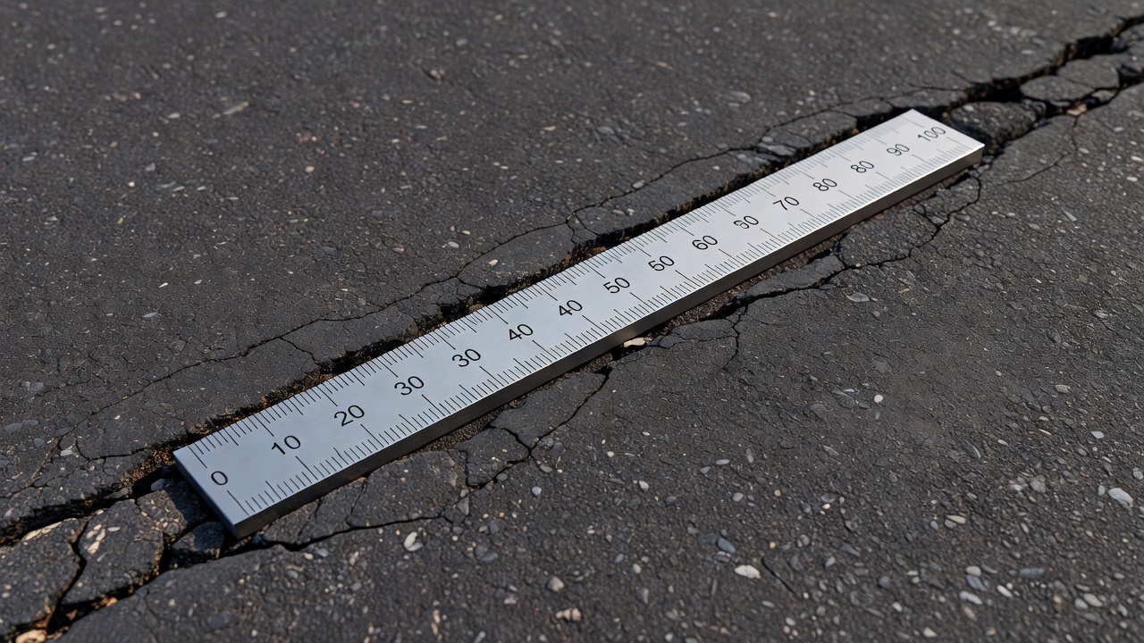
The known reference object method is the simplest, most direct, and most widely used calibration approach. A physical object of precisely known real-world dimensions is placed within the image frame, and its pixel dimensions are measured to compute the scale factor.
Procedure: A reference object with known metric dimensions is placed on the pavement surface within the camera’s field of view. The object should lie in the same plane as the features being measured (coplanar with the pavement surface) and should be oriented parallel to the image plane to avoid foreshortening. The object’s pixel width is measured using image processing techniques (manual measurement, edge detection, or automated feature recognition), and the calibration factor is computed as S = known_length / pixel_length.
Reference object types include:
Scale bars — precision-machined aluminum or carbon fiber bars with calibrated markings at known intervals. A 1-meter scale bar with 1 mm graduations provides calibration traceable to national measurement standards. Scale bars should be rigid, thermally stable (low coefficient of thermal expansion), and have high-contrast markings for reliable automated detection.
Circular coded targets — retroreflective or high-contrast circular targets with known center-to-center distances. Photogrammetric coded targets have the advantage that they can be automatically detected and identified by SfM software, enabling automated calibration without manual measurement.
Pavement markings — standard-width lane markings, runway edge stripes, or taxiway centerline markings provide convenient calibration references when their dimensions are known from design specifications. Per ICAO Annex 14, runway side stripe marking width is 0.9 m (standard) and taxiway centerline marking width is 150 mm. However, pavement markings can wear, spread, or be repainted to non-standard widths, so their actual dimensions should be field-verified before use as calibration references.
Known-dimension pavement features — manhole covers (typically 600-800 mm diameter for airport aprons), runway light fixtures (standardized dimensions per ICAO), joint spacing in concrete pavements (typically 4.5-6.0 m for airfield pavements), and wheel track spacing (standard 1.5-2.0 m for most passenger aircraft and inspection vehicles).
Accuracy considerations: The reference object should span at least 25% of the image dimension in the direction of measurement to keep relative measurement error below 1%. A 100 mm reference object in a 4,000-pixel-wide image covers 400 pixels — a 1-pixel measurement error in the reference contributes only 0.25% calibration error. The same 100 mm reference in a 1,000-pixel image covers only 100 pixels — a 1-pixel error contributes 1% calibration error.
When the camera height above the target surface and the lens focal length are precisely known, the GSD can be calculated directly without a physical reference object in the scene. This method is the standard approach for drone-based orthomosaic generation and for vehicle-mounted line-scan imaging systems.
Calculation method: For a nadir-viewing camera, GSD = (sensor_pixel_pitch × height) / focal_length. For oblique cameras, the effective GSD varies across the image and must be corrected using the camera pose angles (omega, phi, kappa) and the surface geometry.
Height determination — the critical input parameter. For drone surveys, the height above ground is measured by: (1) RTK/PPK GNSS onboard the drone providing ellipsoidal height, corrected using a geoid model to orthometric height above ground; (2) barometric altimeter, which is less accurate (typically ±1-3 m) and sensitive to temperature; (3) laser rangefinder or ultrasonic sensor pointing downward, providing direct height measurement with ±2-10 cm accuracy; (4) LiDAR co-registration where the laser scanner provides per-point distance measurements.
RTK/PPK accuracy: Modern drones equipped with RTK GNSS (such as the DJI Matrice 300 RTK with Zenmuse P1) achieve vertical position accuracy of 2-5 cm RMS when connected to a ground base station or NTRIP correction service. At a 50 m flying height, this 5 cm vertical uncertainty translates to 0.1% GSD uncertainty — negligible for most pavement measurement applications.
Practical limitation: This method requires that the camera is precisely nadir (pointing straight down) or that the camera pose is known and compensated. A 2° tilt from nadir introduces approximately 3.5% GSD variation across the image width for a typical 24 mm lens on full frame — enough to cause significant measurement error in crack width assessment if unaccounted for.
LiDAR co-registration is the most advanced and accurate calibration method, fusing distance measurements from a laser scanner with image data to provide per-pixel scale information across the entire image. This method is used in the most sophisticated vehicle-mounted and drone-based inspection systems.
How it works: A LiDAR scanner (either integrated with the camera or separately mounted and calibrated) captures a dense 3D point cloud of the pavement surface simultaneously with image acquisition. Each LiDAR point has precise 3D coordinates in a real-world coordinate system. Through a process called sensor fusion or calibration registration, each pixel in the image is mapped to its corresponding 3D point. The distance between adjacent pixels in 3D space is computed from the LiDAR data, providing a per-pixel mm/pixel calibration factor.
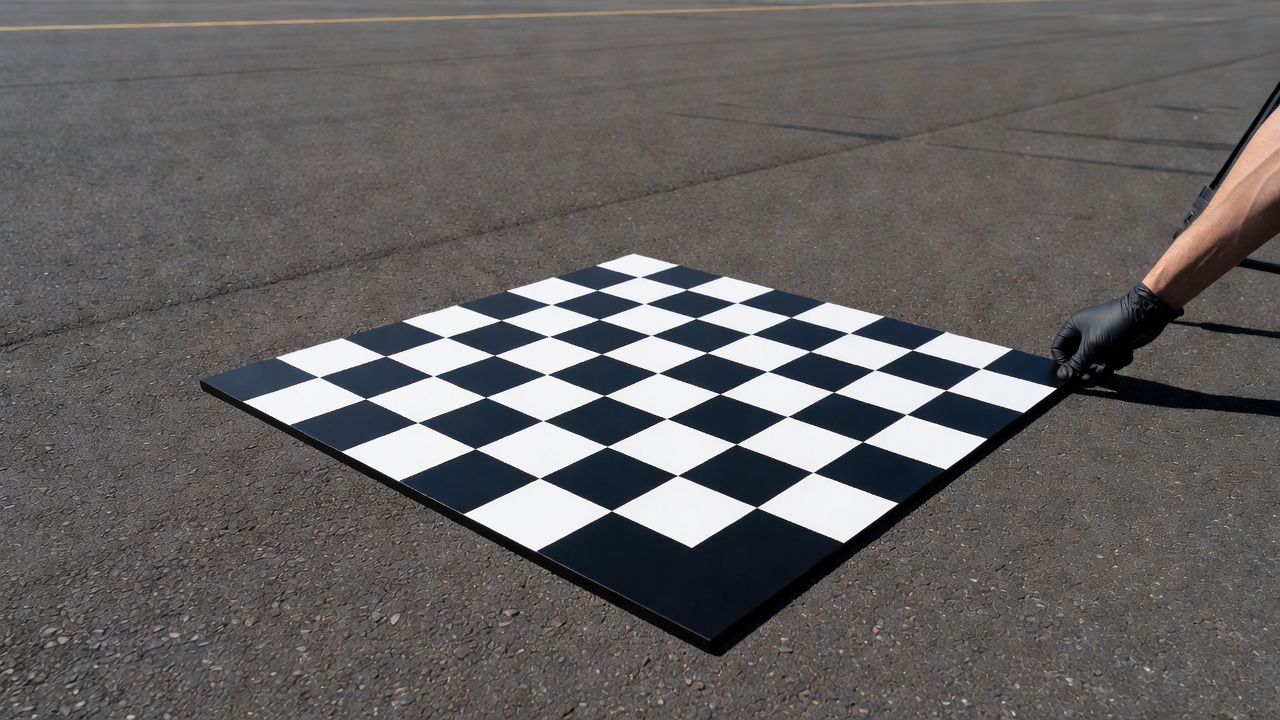
LiDAR-camera calibration requires determination of the rigid transformation (rotation and translation) between the LiDAR sensor coordinate frame and the camera coordinate frame. This is accomplished through target-based calibration using checkerboard patterns visible in both LiDAR intensity data and camera imagery, or through targetless calibration using mutual information maximization and RANSAC-based correspondence matching between edge features.
Advantages: LiDAR co-registration provides calibration for every pixel in the image, automatically correcting for: (1) perspective distortion from oblique camera angles, (2) terrain relief (elevation changes across the pavement surface), (3) camera lens distortion, and (4) rolling shutter effects in line-scan and global shutter cameras. The calibration is traceable to the LiDAR’s distance measurement standard, which itself is calibrated against national standards through the laser time-of-flight measurement.
Accuracy: State-of-the-art LiDAR-camera calibration achieves pixel-level alignment accuracy of 0.3-1.0 pixels for co-registered systems. The resulting per-pixel mm/pixel calibration accuracy is typically 0.2-0.5% of the measured distance for vehicle-mounted systems operating at 1-3 m range, and 0.5-1.0% for drone-based systems operating at 10-50 m range.
Use in TarmacView: TarmacView’s vehicle-mounted pavement inspection system integrates a high-resolution line-scan camera with a 3D LiDAR profiler. The LiDAR provides continuous per-pixel scale calibration across the full pavement width, enabling crack width measurement accuracy of ±0.1 mm at typical survey speeds of 60-80 km/h. The LiDAR also provides rut depth and texture measurements that are spatially correlated with the crack data.
The selection of appropriate reference objects is a critical decision in pixel-to-metric calibration. The reference object establishes the traceability chain from the image measurement back to national measurement standards, and its quality directly determines calibration accuracy.
Scale bars are the gold standard for calibration reference. A precision scale bar consists of a rigid substrate (invar alloy, carbon fiber, or anodized aluminum) with markings at accurately known intervals. Professional photogrammetric scale bars are certified to national standards with length uncertainty of ±0.01 mm/m or better. The scale bar should be placed in the image plane (on the pavement surface) and oriented in the primary direction of measurement. For crack width measurement, the scale bar should be oriented perpendicular to the dominant crack direction. For area measurement, two scale bars at right angles or a single bar oriented at 45° to both axes is recommended.
Circular coded targets are the standard reference in automated photogrammetry. These targets have a precisely known center location defined by concentric black and white rings, with a coded ring pattern that uniquely identifies each target. The targets are surveyed with GNSS or total station to establish their real-world coordinates, and their pixel positions are automatically detected by photogrammetry software to sub-pixel accuracy (typically 0.05-0.1 pixels). A pair of coded targets with known separation distance provides the mm/pixel calibration for the image.
Known-dimension pavement features serve as convenient but less accurate reference objects. Runway centerline markings per ICAO Annex 14 have a standard width depending on the code number: Code 3/4 runways have centerline markings 0.3 m wide for precision runways and 0.15 m for non-precision. Taxiway edge markings are 0.15 m wide. However, actual marking widths can vary by ±10-20% from standard due to wear, repainting, or construction tolerances. Using pavement markings as calibration references requires field verification of their actual dimensions.
When the camera optical axis is not perpendicular to the pavement surface (non-nadir viewing), perspective distortion causes the mm/pixel calibration factor to vary across the image. This is the most significant source of calibration error in practical pavement inspection and the most commonly overlooked.
The geometry of perspective distortion: For a camera tilted by angle θ from the surface normal (0° = nadir, pointing straight down), the effective GSD at a pixel offset x from the image center projected onto the ground is:
GSD_local = GSD_nadir / cos²(θ + arctan(x/f))
Where GSD_nadir is the GSD at the nadir point (directly below the camera), θ is the camera tilt angle, x is the pixel offset from the image center, and f is the focal length. This relationship produces rapid GSD variation across the image:
For a typical oblique drone inspection capturing pavement at 30° from nadir with a 35 mm lens on a full-frame camera, a crack that measures 10 pixels wide at the near edge of the image (where GSD = 1.5 mm/pixel) measures 15 mm wide, while the same physical crack at the far edge (where GSD = 2.6 mm/pixel) measures only 5.8 pixels. Using a single calibration factor for the entire image would produce a 73% measurement error.
Orthorectification is the standard correction for perspective distortion. The raw oblique image is reprojected onto a digital surface model (DSM) of the pavement to produce an orthomosaic with uniform scale. This process requires: (1) accurate camera pose (position and orientation) from GNSS/IMU, (2) a DSM of the pavement surface, (3) camera calibration parameters including lens distortion, and (4) a 3D-to-2D transformation computed for each pixel. The resulting orthomosaic has consistent GSD across the entire image, enabling direct metric measurement.
Homography transformation corrects perspective distortion for planar surfaces (which pavement approximates). The homography matrix H maps points from the distorted image plane to the rectified image plane. For pavement surfaces that are approximately planar (within the image footprint), a single homography correction is sufficient. The homography is computed from four or more reference points with known positions, or from the camera pose using:
H = K × R × K⁻¹
Where K is the camera calibration matrix (intrinsic parameters) and R is the rotation matrix from camera to surface coordinates. However, pavement surfaces are never perfectly planar — even a 2° cross-slope (standard for airport runways per ICAO) introduces measurable elevation differences across the image footprint.
Per-pixel calibration from LiDAR co-registration provides the most rigorous correction, assigning an individual mm/pixel value to every pixel based on the actual 3D distance to the surface measured at that point.
TarmacView implements pixel-to-metric calibration through multiple complementary mechanisms, designed to accommodate the diverse data sources used in pavement inspection.
For direct user-specified calibration, TarmacView accepts the –mm-per-pixel flag that allows the operator to specify the scale factor explicitly. This flag accepts a floating-point value representing millimeters per pixel for the input imagery. When this flag is provided, TarmacView uses the specified calibration factor for all measurement computations, bypassing automated calibration detection.
Usage context: The –mm-per-pixel flag is typically used when: (1) the calibration factor has been determined externally through field measurement with a scale bar, (2) the orthomosaic GSD is known from the processing software but not embedded in the file metadata, (3) the operator wants to override the automated calibration with a manually verified value, or (4) batch processing multiple images that share the same calibration factor.
Validation: When –mm-per-pixel is specified, TarmacView performs consistency checks by detecting known-dimension features in the imagery (lane markings, runway markings) and comparing the measured pixel width against the expected width computed from the specified calibration. If a discrepancy exceeding 10% is detected, a warning is issued and the measurement report flags the potential calibration error.
For orthomosaic inputs with embedded georeferencing metadata, TarmacView extracts the GSD directly from the GeoTIFF file. GeoTIFF files store spatial resolution information in their metadata tags (ModelTiepointTag and ModelPixelScaleTag for GSD, or ModelTiepointTag and ModelTransformationTag for more complex coordinate systems). The platform reads these tags and computes the effective mm/pixel factor for the orthomosaic.
For raw (non-orthorectified) imagery, TarmacView’s automated pipeline detects reference objects in the scene including: (1) coded photogrammetric targets with known dimensions, (2) scale bars with high-contrast markings, (3) pavement markings whose standard dimensions are stored in the platform’s reference database, and (4) repetitive pavement features (joint spacing, light fixture spacing) with known dimensions. The detected reference provides the calibration factor for that image.
For TarmacView’s vehicle-mounted inspection system, which combines line-scan cameras with 3D LiDAR profilers, the calibration is computed per-pixel from the LiDAR distance measurements. The LiDAR profiler provides a continuous cross-section of the pavement surface at 1-5 mm lateral resolution, with each point carrying accurate 3D coordinates. The camera image is co-registered with the LiDAR data through a factory-calibrated rigid transformation. Each pixel in the camera image is mapped to its corresponding LiDAR 3D point, and the mm/pixel factor for that pixel is computed from the 3D distance between adjacent LiDAR points projected into the image coordinate system. This approach automatically accounts for camera perspective, lens distortion, terrain relief, and vehicle motion.
The calibration factor is not a single deterministic value — it carries uncertainty that propagates through all subsequent measurements. Understanding and quantifying this propagation is essential for reliable pavement condition assessment.
The total uncertainty in any image-based metric measurement has three components:
Calibration uncertainty (u_cal) — the uncertainty in the mm/pixel factor. Sources include: (1) reference object dimension uncertainty (typically ±0.1-0.5% for certified scale bars), (2) reference object pixel measurement uncertainty (typically ±0.3-1.0 pixels for manual measurement, ±0.05-0.3 pixels for automated sub-pixel detection), (3) perspective distortion uncertainty (residual errors after orthorectification or homography correction), (4) lens distortion uncertainty (residual distortion after calibration), and (5) height measurement uncertainty (for the GSD formula method).
Measurement uncertainty (u_meas) — the uncertainty in locating the feature boundaries in the image. For crack width measurement, this is the uncertainty in the edge detection algorithm. Sub-pixel edge detection methods (interpolation, moment-based, or Gaussian fitting) typically achieve 0.1-0.3 pixel precision. Manual measurement by a human operator typically achieves 0.5-1.0 pixel precision. The measurement uncertainty in metric units is u_meas × S (the mm/pixel factor).
Sample uncertainty (u_sample) — the uncertainty from sampling a variable feature. Crack width varies along the crack length. A single measurement is not representative of the whole crack. ASTM D5340 requires measurement at the representative width of each distress severity level, which introduces sampling uncertainty. For area measurement, the boundary delineation uncertainty affects the computed area through the perimeter-to-area ratio.
For a crack measured as having w_pixels pixel width, the metric crack width is:
w_mm = S × w_pixels
The combined standard uncertainty is:
u_w = w_mm × sqrt[(u_cal/S)² + (u_meas/w_pixels)²]
Example: A crack measures 8 pixels wide at a calibration factor of S = 0.5 mm/pixel (w_mm = 4.0 mm). The calibration uncertainty is u_cal = 0.005 mm (1% of S), and the edge detection uncertainty is u_meas = 0.2 pixels.
u_w = 4.0 × sqrt[(0.005/0.5)² + (0.2/8)²] = 4.0 × sqrt[0.0001 + 0.000625] = 4.0 × 0.027 = 0.11 mm
The expanded uncertainty at 95% confidence (coverage factor k=2) is ±0.22 mm, or ±5.5% of the crack width. This crack can be confidently classified as “severe” (>3 mm per ASTM D5340).
For a narrower crack measuring 3 pixels at the same calibration: w_mm = 1.5 mm, u_w = 1.5 × sqrt[(0.01)² + (0.067)²] = 1.5 × 0.068 = 0.10 mm. The expanded uncertainty is ±0.20 mm (k=2), or ±13.3% of the crack width. This crack could be 1.3-1.7 mm, which straddles the classification boundary between “low severity” (<1 mm) and “medium severity” (1-3 mm).
Crack length measurement uncertainty combines the calibration uncertainty with the path tracing uncertainty. For a crack composed of n pixel-length segments forming a continuous path:
L_mm = S × n
The uncertainty is dominated by the path tracing uncertainty (how accurately the crack centerline is followed) plus the calibration uncertainty:
u_L = L × sqrt[(u_cal/S)² + (u_trace/n)²]
Where u_trace is the path tracing uncertainty in pixels per segment (typically 0.3-0.5 pixels for automated tracing, 0.5-1.5 pixels for manual tracing). For a 3 m crack (6,000 pixels at 0.5 mm/pixel) traced automatically with u_trace = 0.4 pixels/segment, the length uncertainty is approximately ±0.04 m (k=2) — about 1.3% relative uncertainty.
Area measurement uncertainty is more complex because it combines calibration uncertainty in two dimensions plus boundary delineation uncertainty. For a spalled area measured from an orthomosaic:
A_mm² = S² × A_pixels
The relative uncertainty in area is approximately:
u_A/A = sqrt[4 × (u_cal/S)² + (2 × u_boundary / perimeter)²]
Where u_boundary is the boundary delineation uncertainty in pixels and perimeter is the spall perimeter in pixels. For a 0.5 m² spall (20,000 pixels at 1 mm/pixel, perimeter ~600 pixels) with u_cal = 0.01 mm (1%) and u_boundary = 1.0 pixel:
u_A/A = sqrt[4 × (0.01)² + (2 × 1 / 600)²] = sqrt[0.0004 + 0.000011] = 0.0203
The expanded area uncertainty at 95% confidence is ±0.020 m², or ±4.1% relative uncertainty.
| Measurement | Typical Relative Uncertainty (k=2, 95% confidence) | Calibration Contribution | Measurement Contribution |
|---|---|---|---|
| Crack width >3 mm (GSD 0.5 mm/px) | ±5-10% | ±1-2% | ±4-8% |
| Crack width <1 mm (GSD 0.5 mm/px) | ±15-30% | ±1-2% | ±14-28% |
| Crack length (GSD 1 mm/px) | ±2-5% | ±1-2% | ±1-3% |
| Spalled area 0.5 m² (GSD 1 mm/px) | ±4-8% | ±2-4% | ±2-4% |
| Rut depth (LiDAR co-registered) | ±2-4% | ±0.5-1% | ±1.5-3% |
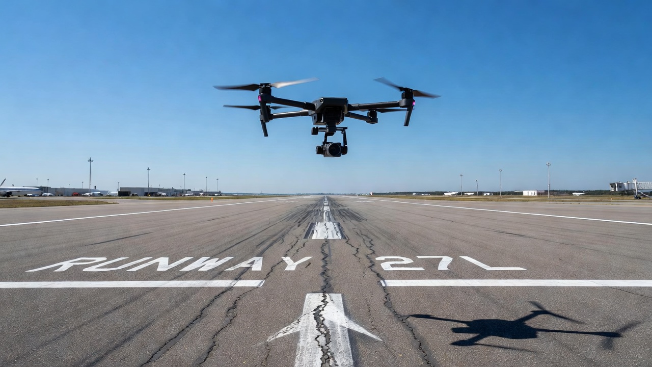
Drone-based pavement inspection presents specific calibration challenges related to flight altitude variability, camera motion, and large-area coverage.
For a typical drone survey covering 10-50 hectares of pavement, the flying height varies due to terrain elevation changes, atmospheric conditions, and GNSS altitude uncertainty. A 2 m height variation on a 50 m survey altitude produces 4% GSD variation — enough to affect crack width classification boundaries. The standard correction is to compute a GSD surface — a raster dataset where each pixel value is the local GSD computed from the DSM elevation and the camera pose for the image covering that pixel.
In photogrammetric surveys with 80-90% forward overlap and 70-80% side overlap, every point on the ground appears in 5-15 overlapping images, each with slightly different camera-to-surface geometry. The redundant coverage enables multi-image averaging of measurements, reducing the effective measurement uncertainty. For crack width measurement from an orthomosaic derived from multiple images, the uncertainty is reduced by approximately sqrt(n), where n is the number of contributing images at that location.
Ground control points (GCPs) serve a dual purpose in drone surveys: they establish absolute georeferencing accuracy and provide the reference distances for mm/pixel calibration validation. A minimum of 5-8 GCPs distributed across the survey area is recommended for calibration validation. The distance between GCP pairs is a known surveyed value, and comparison with the image-measured distance (in pixels) provides an independent calibration check. Residual analysis of GCP distances reveals whether the calibration is consistent across the survey area or whether systematic errors (e.g., uncorrected lens distortion, DEM errors) are present.
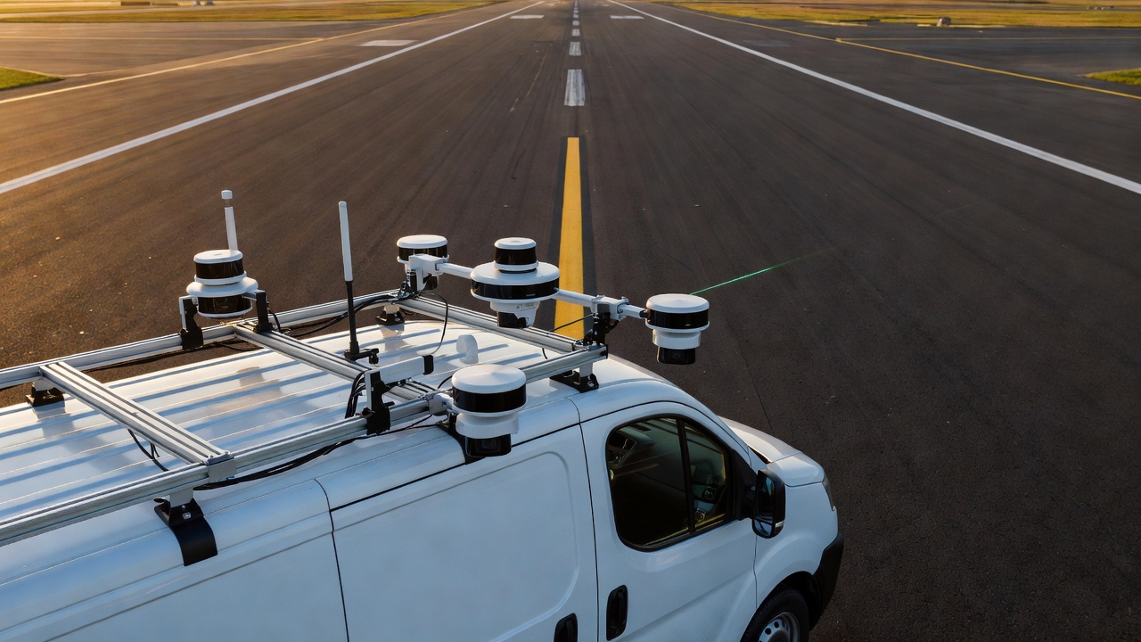
Vehicle-mounted pavement inspection systems operate at much closer range (1-4 m above the pavement) and higher speeds (60-100 km/h), creating distinct calibration requirements compared to drone-based systems.
Vehicle-mounted systems often use line-scan cameras (also called push-broom cameras) that capture a single line of pixels at a time. The forward motion of the vehicle provides the second spatial dimension. The calibration for line-scan cameras requires:
Lateral calibration — the mm/pixel factor across the pavement width (perpendicular to travel direction). This depends on the camera height above pavement and the lens focal length. For a camera mounted at 2.5 m height with a 16 mm lens and 7 μm pixel pitch, the lateral GSD is (0.007 × 2500) / 16 = 1.1 mm/pixel at the nadir line. At the edges of a 6 m wide pavement (3 m from nadir), perspective distortion increases the lateral GSD to approximately 1.4 mm/pixel — a 27% variation that must be corrected.
Longitudinal calibration — the mm/pixel factor along the travel direction. This is determined by the vehicle speed and the line-scan camera’s line rate (lines per second). Each line of pixels is triggered by an encoder wheel or by time-based triggering synchronized to vehicle speed. An encoder wheel with 1,000 pulses per revolution on a 0.5 m circumference wheel provides 0.5 mm/pulse resolution. Line triggering at every 2 encoder pulses produces 1.0 mm longitudinal pixel spacing at any vehicle speed. Calibration of the encoder wheel circumference (which changes with tire pressure and wear) is critical — a 2% tire circumference error (typical from inflation variation) produces a 2% longitudinal measurement error.
Vehicle bounce, pitch, and roll from pavement roughness cause camera height variation at frequencies of 1-10 Hz with amplitudes of 2-20 mm on typical pavement surfaces. These motions introduce time-varying calibration errors that must be corrected through: (1) a laser height sensor measuring instantaneous camera-to-pavement distance at 100-1000 Hz, (2) an inertial measurement unit (IMU) measuring vehicle body accelerations and angular rates, (3) post-processing correction using a Kalman filter or complementary filter that fuses the laser height, IMU, and encoder data to compute per-line calibration factors.
The required calibration accuracy depends on the measurement application and the criticality of the pavement distress classification thresholds.
ASTM D5340 (Standard Test Method for Airport Pavement Condition Index Surveys) defines crack width thresholds at 1 mm, 3 mm, and 6 mm for classifying crack severity in both asphalt and concrete pavements. To reliably distinguish a 2.9 mm crack (just below the 3 mm severe threshold) from a 3.1 mm crack (just above it), the measurement uncertainty must be less than ±0.1 mm at 95% confidence — requiring calibration uncertainty below 2% for the typical crack width range.
ICAO Annex 14 specifies geometric tolerances for pavement surfaces including surface flatness, cross-slope, and longitudinal grade. While these are primarily construction tolerances, they establish the expectation for survey-grade measurement accuracy in pavement inspection.
ISO/TS 19159-1 (Geographic information — Calibration and validation of remote sensing imagery sensors and data) provides the framework for calibration uncertainty assessment and reporting, including calibration hierarchy, traceability chain, and uncertainty budget requirements.
FHWA-RC-20-0005 (Evaluation of Crack Measurement Methods for Pavement Condition Assessment) establishes a statistical framework for evaluating crack measurement systems, requiring independent validation with reference measurements and reporting of bias and precision at specified confidence levels.
| Application | Required GSD | Required Calibration Accuracy | Reference Method |
|---|---|---|---|
| Precision crack width measurement | ≤0.5 mm/pixel | ±0.5% | Scale bar + sub-pixel detection |
| Standard crack width classification | ≤1.5 mm/pixel | ±2% | GCP distances or GSD calculation |
| Crack length mapping | ≤3 mm/pixel | ±5% | Standard reference object |
| Spalled area measurement | ≤2 mm/pixel | ±3% | Two orthogonal scale bars |
| Rut depth (from orthomosaic) | ≤2 mm/pixel (vertical) | ±2% | LiDAR co-registration |
| PCI survey (all distress types) | ≤3 mm/pixel | ±5% | Surveyed GCPs |
Always verify calibration in the field. Photograph a certified scale bar in the same plane and lighting as the pavement being inspected. The scale bar should be placed at multiple locations across the survey area to verify calibration consistency. For drone surveys, include a scale bar in at least one image per flight line.
Use sub-pixel measurement for reference objects. Automated target detection with sub-pixel accuracy (0.05-0.3 pixels) reduces calibration uncertainty by 3-10× compared to manual pixel counting. Circular coded targets with center-weighted centroid detection routinely achieve 0.05-0.1 pixel accuracy.
Account for terrain relief. Pavement surfaces are never perfectly flat. Runway cross-slope (1.5-2.5% standard), longitudinal grade (0-2% standard), and local depressions from settlement or rutting cause elevation differences that affect calibration. Use a DSM or local height measurements to correct for terrain effects.
Document the calibration traceability chain. Record the reference object certification, measurement method, operator, date, environmental conditions (temperature affects scale bar length by 0.01 mm/m/°C for aluminum bars), and all uncertainty components. This documentation is essential for quality assurance, audit compliance, and legal defensibility of measurements.
Perform independent validation. After calibration, measure an independent check object (different from the calibration reference) and compare the image measurement with its known dimension. The discrepancy should be within the expected uncertainty. Repeat this validation at least once per survey session and whenever the imaging setup changes.
Monitor calibration stability. For fixed imaging systems (vehicle-mounted cameras, permanent installation cameras), perform daily calibration verification using a built-in reference target. Record calibration values over time to detect drift from temperature effects, mechanical wear, or component degradation. A calibration drift exceeding 2% from the baseline value should trigger recalibration and investigation.
Report calibration uncertainty with every measurement. Pavement condition reports should include the calibration method, the calibration factor, its uncertainty, and the resulting measurement uncertainty for each reported distress value. This enables the asset manager to make risk-informed decisions — a crack width reported as “3.0 mm ± 0.2 mm” carries different operational implications than one reported as “3.0 mm ± 1.5 mm.”
Pixel-to-metric calibration expressed as millimeters per pixel (mm/px) is the foundational transformation that enables quantitative image-based pavement measurement. Without accurate calibration, crack width, crack length, and spalled area remain dimensionless pixel counts that cannot be compared to PCI severity thresholds, ICAO pavement condition criteria, or maintenance priority matrices. The calibration factor is determined through three primary methods — known reference objects, camera height and field of view calculation, and LiDAR co-registration — each with specific accuracy characteristics and operational tradeoffs. Perspective distortion from oblique camera angles is the most significant source of calibration error, requiring orthorectification, homography correction, or per-pixel LiDAR-based calibration for reliable results. Calibration uncertainty propagates through all derived measurements and must be quantified and reported with every distress measurement. The recommended calibration accuracy for PCI-compliant crack width classification is ±2% (standard) to ±0.5% (precision), achievable through proper use of certified reference objects, sub-pixel measurement techniques, and rigorous quality control procedures. TarmacView implements these calibration principles through its –mm-per-pixel flag, automated orthomosaic GSD extraction, LiDAR co-registration pipeline, and full uncertainty propagation to all measurement outputs.
TarmacView's automated pixel-to-metric calibration pipeline delivers traceable, survey-grade crack width measurements from drone and vehicle-mounted imagery. Generate ASTM-compliant PCI reports with verified mm/pixel calibration and full uncertainty propagation.
Automated crack width measurement derives the opening width of detected cracks from segmented pixel masks using Euclidean distance transform from crack edges to...
Camera calibration determines intrinsic parameters (focal length, principal point, lens distortion coefficients) essential for accurate photogrammetric measurem...
A pavement distress survey systematically identifies, classifies, and measures each distress type, severity, and extent on a pavement section following standard...