Camera Calibration

What is Camera Calibration?

Camera calibration is the process of determining the geometric parameters that define how a camera maps 3D world coordinates to 2D image coordinates. It answers a deceptively simple question: given a point in the real world (x, y, z), which pixel (u, v) in the image does it map to, and with what mathematical precision?

At its core, calibration exists because cameras are imperfect implementations of the ideal pinhole model. Every real camera-lens system deviates from perfection in ways that must be characterized and corrected before the camera can be used as a measurement instrument. Without calibration, every distance, area, and volume derived from images carries unquantified systematic error — the very thing that distinguishes photogrammetry from casual photography.

The Pinhole Camera Model

The pinhole camera model is the mathematical foundation upon which all camera calibration is built. It describes the ideal projective transformation from 3D world coordinates to 2D image coordinates through a single point — the center of projection (camera center). The model assumes that light travels in straight lines through an infinitesimally small aperture, that there is no lens, and that the image plane is perfectly planar and orthogonal to the optical axis.

Under the pinhole model, a 3D point X = [X, Y, Z, 1]ᵀ in world coordinates maps to image point x = [u, v, 1]ᵀ through the projection equation λx = K[R|t]X, where λ is a scale factor (the projective depth), K is the 3×3 intrinsic camera matrix, and [R|t] is the 3×4 extrinsic matrix representing rotation and translation from world to camera coordinates. Real lenses introduce systematic deviations from this ideal model — deviations that calibration quantifies and corrects.

Why Calibration Matters

An uncalibrated camera is not a measurement device. Consider what happens when a pavement inspection camera with a wide-angle lens captures an image of a road surface. Barrel distortion pulls pixels near the image edges inward by tens of pixels. Without a distortion model, a 0.3 mm crack at the image edge might appear as a 0.2 mm or 0.4 mm feature — or be invisible entirely. The principal point may be offset from the image center by 5-15 pixels due to manufacturing tolerances. Focal length, often assumed from the lens specification, can differ by 2-5% from the nominal value.

These seemingly small errors compound catastrophically in measurement. A 1% error in focal length translates to a 1% error in all derived distances. A 10-pixel principal point offset at a ground sample distance (GSD) of 1 mm/pixel introduces a 10 mm systematic shift in all measurements. Distortion of 5 pixels at the image edge translates to 5 mm of error at the corresponding ground location.

The Intrinsic Matrix K

The intrinsic matrix K encodes the internal geometric properties of a camera. It is a 3×3 upper-triangular matrix that maps 3D camera-centered coordinates to 2D pixel coordinates:

    [ fx   s   cx ]
K = [  0   fy  cy ]
    [  0    0   1 ]

Focal Length (fx, fy)

The focal length parameters fx and fy represent the distance from the camera center to the image plane, expressed in pixels. In an ideal camera, fx = fy. Differences arise from non-square pixels, sensor manufacturing tolerances, and anamorphic lens elements.

Conversion between pixel and physical units: The focal length in millimeters F can be computed from the pixel focal length as Fx = fx × (W/w), where W is the sensor width in mm and w is the image width in pixels. For a 24 MP camera with a 24 mm lens, 6 μm pixel pitch (6000 × 4000 pixels on a 36 × 24 mm sensor), the focal length in pixels is approximately 4000 pixels.

Principal Point (cx, cy)

The principal point is the intersection of the optical axis with the image sensor — the point in the image where the camera’s optical axis pierces the image plane. In an ideal camera, it sits at the geometric center of the sensor: cx = w/2, cy = h/2. In real cameras, manufacturing tolerances shift it by 1-15 pixels from center. For the 24 MP example, cx ≈ 3000 pixels, cy ≈ 2000 pixels.

The principal point serves as the origin for lens distortion calculations — distortion displacements are measured radially from this point. A misidentified principal point causes distortion correction to be applied around the wrong center, introducing systematic errors that increase with distance from the true principal point.

Skew Coefficient (s)

The skew coefficient s accounts for non-rectangular pixels — a shear distortion in the image plane. In modern digital cameras with orthogonal sensor grids and rectangular pixels, the skew is effectively zero (s = 0). Historical analog cameras and certain scanning systems could exhibit non-zero skew, but for virtually all digital inspection cameras, skew can be assumed zero.

Lens Distortion Models

Lens distortion is the systematic deviation of real lens geometry from the ideal pinhole projection. The International Society for Photogrammetry and Remote Sensing (ISPRS) and the computer vision community have standardized on the Brown-Conrady model as the primary mathematical framework for describing lens distortion.

Radial Distortion (k1, k2, k3)

Radial distortion displaces image points along radial lines extending from the principal point. It is caused by the spherical shape of lens elements — light rays passing through the periphery of a spherical lens are refracted differently than rays through the center. The distortion is modeled as a polynomial function of the radial distance r from the principal point:

x_undistorted = x × (1 + k₁r² + k₂r⁴ + k₃r⁶) y_undistorted = y × (1 + k₁r² + k₂r⁴ + k₃r⁶)

Where (x, y) are normalized image coordinates relative to the principal point and r² = x² + y². The coefficient k1 dominates the distortion magnitude, with k2 and k3 providing increasingly subtle higher-order corrections. A negative k1 produces barrel distortion (points displaced inward, image appears bulging), while a positive k1 produces pincushion distortion (points displaced outward, image appears pinched).

For a typical wide-angle lens used in drone inspection (k1 ≈ -0.1), radial displacement at the image corner reaches 40-100 pixels, corresponding to 4-10 cm of measurement error at 1 mm GSD.

Tangential Distortion (p1, p2)

Tangential (decentering) distortion arises from imperfect alignment of individual lens elements in compound lenses — the optical centers of successive elements are not perfectly collinear. The Brown-Conrady model corrects tangential distortion using two parameters:

x_undistorted = x + [2p₁xy + p₂(r² + 2x²)] y_undistorted = y + [p₁(r² + 2y²) + 2p₂xy]

Tangential distortion is typically one to two orders of magnitude smaller than radial distortion for quality lenses. For most infrastructure inspection cameras, p1 and p2 are on the order of 10⁻⁴ to 10⁻⁵, producing displacements of 0.1-0.5 pixels at image corners. However, for lenses that have been physically damaged or poorly assembled, tangential distortion can exceed 5-10 pixels, significantly degrading measurement accuracy.

The Brown-Conrady Full Model

Duane C. Brown (1966, 1971) and A. E. Conrady (1919) developed the complete distortion model that is the standard in both photogrammetry and computer vision. The full model combines radial and tangential components into a single correction applied to each image point. The photogrammetric formulation differs slightly from the computer vision formulation: photogrammetry corrects from distorted to ideal coordinates as a function of distorted coordinates, while computer vision compensates from ideal to distorted as a function of ideal coordinates. This distinction is critical when transferring calibration parameters between photogrammetric (e.g., Agisoft Metashape) and computer vision (e.g., OpenCV) software.

Fisheye Model

For wide field-of-view lenses (≥ 90° field of view), the standard Brown-Conrady model becomes inadequate because the polynomial expansion diverges at large radial distances. The fisheye model uses a different projection function based on the angle θ of the incoming ray:

θ_d = θ(1 + k₁θ² + k₂θ⁴ + k₃θ⁶ + k₄θ⁸)

Where r = tan(θ) for the standard pinhole model, but r = θ (equidistant projection) for the fisheye model. Fisheye calibration typically requires 4 radial parameters (k1-k4) and no tangential parameters. Many consumer drone cameras with wide-angle lenses benefit from fisheye calibration, though the Brown-Conrady model is sufficient for normal and moderate wide-angle lenses (< 90° field of view).

Calibration Methods

Three primary methods dominate camera calibration practice, each with distinct accuracy characteristics, equipment requirements, and workflow implications.

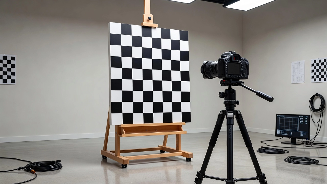
Zhang’s Checkerboard Method

Zhengyou Zhang’s 2000 paper “A Flexible New Technique for Camera Calibration” (IEEE Transactions on PAMI, cited 23,000+ times) introduced the method that has become the de facto standard for camera calibration. Zhang’s method requires only a planar checkerboard pattern printed on a flat surface — no expensive 3D test field or precision optical bench.

Mathematical framework: The method exploits the homography H between a planar calibration pattern (Z=0 in world coordinates) and its image projection. For each image of the checkerboard, the homography is computed from the known corner positions and their detected image coordinates. The homography provides two constraints on the intrinsic parameters via the absolute conic:

h₁ᵀ(A⁻ᵀA⁻¹)h₂ = 0 h₁ᵀ(A⁻ᵀA⁻¹)h₁ = h₂ᵀ(A⁻ᵀA⁻¹)h₂

These constraints follow from the fact that the rotation matrix columns r1 and r2 are orthonormal. With n images, 2n equations are available, and the intrinsic matrix A (equivalent to K) has 5 unknown parameters (fx, fy, cx, cy, s). A minimum of 3 images provides 6 equations for a closed-form solution.

Solution process: The closed-form solution is computed analytically, then refined via maximum likelihood estimation using the Levenberg-Marquardt algorithm. The refinement minimizes the total reprojection error:

min Σᵢⱼ ||pᵢⱼ - p̂(K, Rᵢ, tᵢ, Pⱼ)||²

where pᵢⱼ is the detected corner j in image i, and p̂ is the projected corner from the model. Radial distortion parameters (k1, k2) are typically added to the optimization in a second stage.

Pattern requirements: For reliable results, the checkerboard must satisfy flatness < 0.1 mm, a pattern size of 7×10 to 9×12 corners, square size of 10-30 mm, and 10-20 images at varied orientations. Images must cover all sensor quadrants including corners and edges, as the distortion model is poorly constrained without corner data.

Degenerate configurations: The method fails if the pattern undergoes pure translation (no rotation between images) or if all images are captured with the pattern parallel to the image plane. This is why calibration requires tilting and rotating the checkerboard between captures.

3D Test Field Calibration

Before Zhang’s method, calibration was performed using precisely surveyed 3D test fields — arrays of targets with known coordinates occupying a defined volume. The camera photographs the test field from multiple positions, and the known 3D-to-2D correspondences directly constrain all calibration parameters. This method achieves the highest accuracy (< 0.1 pixels RMS) but requires expensive surveying equipment, physical space, and maintenance. It remains the gold standard for metrology applications where maximum accuracy is required and budget permits.

Self-Calibration in Bundle Adjustment

Self-calibration (on-the-job calibration) estimates camera parameters simultaneously with 3D reconstruction during bundle adjustment. This approach is central to modern Structure from Motion (SfM) pipelines including Agisoft Metashape, Pix4Dmapper, COLMAP, and RealityCapture.

How it works: The pipeline detects thousands of tie points across overlapping images using feature detectors (SIFT, AKAZE, SuperPoint). A rough camera model is initialized from EXIF metadata. Bundle adjustment then simultaneously refines camera intrinsics (K, distortion coefficients), camera extrinsics (R, t for each image), and 3D point coordinates (Xⱼ) by minimizing the total reprojection error across all observations.

Critical requirements: Self-calibration requires convergent images (non-parallel optical axes), orthogonal roll angles, full image coverage (especially edges and corners), and for flat terrain, oblique images at 20-45° off-nadir. Without these conditions, the estimation problem is ill-posed — radial distortion parameters become strongly correlated with elevation, producing the dome effect.

Pre-Calibrated vs On-the-Job Calibration

A fundamental decision in photogrammetric workflow design is whether to pre-calibrate the camera in a controlled environment or to rely on on-the-job self-calibration.

For rectangular nadir-only blocks typical of infrastructure inspection, pre-calibration provides more accurate results because the block geometry is insufficient to decorrelate distortion parameters from elevation. The accuracy gap narrows significantly when adequate ground control points (GCPs) are distributed at block boundaries and centers. The optimal approach combines both methods: pre-calibrate the camera in a laboratory setting using Zhang’s method, then allow self-calibration refinement in the SfM pipeline only when the block includes oblique images (≥10% of images at 20-45° tilt).

Calibration Stability Over Time

Camera calibration parameters are not permanent. Thermal effects, mechanical shocks, and aging cause them to drift.

Thermal Effects

Temperature changes cause measurable geometric drift in consumer cameras. Research published in MDPI Sensors (2017) demonstrated focal length drift of 0.01-0.05% per °C. For a 4000-pixel focal length, this translates to 0.4-2.0 pixels per 10°C change. Principal point shifts of 0.1-0.5 pixels per °C are typical, and the dominant radial distortion coefficient k₁ can vary by 1-5% over a 30°C range. A drone taking off at 25°C and climbing to operating altitude where the temperature is 10°C experiences a 15°C change, causing focal length drift equivalent to 6-30 pixels or 1.5-7.5 mm of measurement error at 1 mm GSD. Photogrammetric accuracy improves by 2-4× when thermal effects are modeled and compensated.

Mechanical Shocks

Consumer-grade cameras are geometrically fragile. Dropping a camera can shift the principal point by 1-10 pixels. Removing and reattaching interchangeable lenses can alter the flange focal distance, shifting the principal point by 2-5 pixels. Auto-focus mechanisms change principal distance with every focus operation. Sensor-shift or lens-shift image stabilization introduces variable geometric offsets and must be disabled for photogrammetric use.

Recalibration Frequency

Effects of Uncalibrated Cameras on Measurements

An uncalibrated camera introduces systematic errors into every derived measurement. Understanding the propagation of these errors is essential for designing inspection workflows that meet accuracy requirements.

The Dome Effect

The dome effect is the most insidious consequence of inadequate calibration in aerial photogrammetry. It manifests as a systematic elevation error where the center of the reconstructed surface is elevated relative to the edges (doming) or depressed relative to the edges (bowling). The causal mechanism is the strong correlation between radial distortion (especially k₁) and elevation in nadir-only imagery — bundle adjustment incorrectly absorbs radial distortion into elevation variations, producing a smooth, systematic error surface that looks realistic but is geometrically wrong. Magnitude: 0.1-0.5% of flight height (10-50 cm at 100 m altitude, 1-5 cm at 20 m altitude). Mitigation strategies include including oblique images at 20-45° off-nadir (at least 10% of block images), distributing GCPs at block boundaries and centers, flying cross strips (double-grid pattern), and using GNSS-assisted camera stations.

Calibration for Close-Range Photogrammetry

Close-range photogrammetry (camera-to-object distances < 300 m) benefits from strongly convergent camera networks where the camera is pointed at the same scene region from multiple directions. The ideal calibration network uses convergent images with 60-120° angle differences, cameras rolled to all four quadrants (0°, 90°, 180°, 270°), and images filling all sensor corners and edges.

Coded targets — circular retroreflective markers with unique identification patterns — provide automatic identification, sub-pixel measurement accuracy (0.01-0.05 pixels centroid), and automated correspondence. Close-range calibration with coded targets consistently achieves RMS reprojection errors below 0.1 pixels and object-space accuracy ratios of 1:50,000 to 1:200,000 (ratio of object size to measurement accuracy).

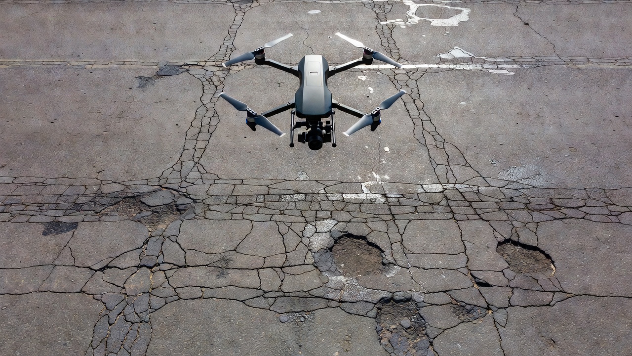
Calibration for Drone/UAV Cameras

Drone-based photogrammetry occupies a challenging middle ground where consumer-grade cameras (borrowing challenges from close-range calibration) meet aerial block geometry (borrowing constraints from aerial photogrammetry). Unique challenges include mechanical instability from hard landings and gimbal shocks, auto-focus that changes principal distance in flight, temperature gradients of 10-40°C between ground and altitude, and CMOS rolling shutter that introduces geometric distortion.

Recommended Flight Configurations

Research by Roncella and Forlani (Sensors, 2021) demonstrated that the accuracy gap between optimal and poor calibration configurations can be close to an order of magnitude for UAV blocks. Self-calibration with oblique images (≥10% of block images at 20-45° tilt) combined with a double-grid flight pattern reduces the dome effect from 0.1-0.5% of flight height to < 0.01%.

Calibration Quality Assessment

A calibration is only as good as its quality assessment. Multiple complementary metrics must be evaluated to determine whether a calibration is fit for purpose.

Reprojection Error

RMS reprojection error (RPE) is the most widely reported calibration quality metric. It measures the 2D pixel difference between detected image features and their positions computed from the camera model and 3D coordinates: RPE = √(1/n × Σ||xᵢ - x̂ᵢ||²).

Critical caveat: RPE is a training error. It measures how well the model fits the data used to estimate it. A low RPE does not guarantee good calibration because of overfitting risk (too many parameters for the available constraints). Always validate with independent check points measured in the calibration images but not used in parameter estimation.

Variance-Covariance Analysis

The variance-covariance matrix Cx = σ₀² × (JᵀJ)⁻¹ provides essential uncertainty information, where σ₀² is the a posteriori variance factor and J is the Jacobian matrix. The standard deviation of each parameter is the square root of the corresponding diagonal element. Parameter significance is assessed using the t-statistic t = |pᵢ| / σ(pᵢ): t > 2.0 indicates significance at 95% confidence.

Correlation Monitoring

The most critical correlation to monitor is between focal length (fx) and radial distortion (k₁):

Correlations above 0.9 between fx and k₁ indicate that the image block lacks oblique views, and self-calibration will produce unreliable results. Pre-calibration or additional oblique images are required.

USGS Guidelines

USGS Open-File Report 2023-1033 requires that all calibration parameters and their uncertainties be reported as metadata, the calibration method and date be documented, the calibration environment (temperature, humidity) be recorded, validation metrics (RPE, check point residuals) be provided, and recalibration history be maintained.

Calibration in Infrastructure Inspection and Crack Measurement

Infrastructure inspection — particularly pavement crack measurement — places stringent demands on camera calibration. Cracks as narrow as 0.1 mm must be reliably detected and measured, requiring sub-millimeter measurement accuracy across large surface areas.

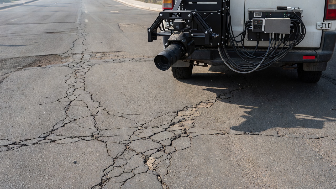
Pavement Inspection Camera Parameters (ISPRS 2025 Study)

A recent ISPRS pavement inspection study (Darwish & Ahmed, 2025) using a vehicle-mounted camera system at 2.237 m height reported the following calibration parameters:

Impact on Crack Measurement

Uncalibrated cameras introduce systematic errors that directly affect crack measurement. A 5-pixel uncorrected barrel distortion at image edges translates to 5 mm error at 1 mm GSD — sufficient to entirely mask sub-millimeter cracks or falsely widen hairline cracks by 200-500%. Principal point errors of 10 pixels introduce 10 mm lateral offsets in crack location. Focal length errors of 2% produce 2% scaling errors in crack width measurements.

Calibration enables three critical transformations for pavement inspection: lens distortion correction (removing barrel/pincushion distortion that would otherwise warp crack geometry at image edges), orthogonal projection (converting perspective images to bird’s-eye orthographic views where true metric measurements are possible), and metric scaling (establishing the precise relationship between pixels and millimeters on the road surface).

Summary and Best Practices

Camera calibration is the foundation of all photogrammetric measurement. Without it, images are qualitative records, not quantitative data. With proper calibration, sub-millimeter measurement accuracy is achievable even with consumer-grade cameras.

Key Takeaways

1. Every camera-lens combination has unique calibration parameters — never assume parameters from the same model or another unit.
2. Calibration parameters drift over time — thermal effects (~0.01-0.05% per °C), mechanical shocks, and aging all degrade calibration validity.
3. Self-calibration is not a silver bullet — without oblique images (20-45°), the correlation between fx and k₁ produces dome effect errors of 0.1-0.5% of flight height.
4. Pre-calibration + self-calibration refinement is the optimal approach — lab calibration provides robust initial values; on-the-job refinement adapts to field conditions.
5. Quality assessment requires multiple metrics — RMS reprojection error alone is insufficient; variance-covariance analysis, parameter significance testing, and independent check point validation are essential.
6. For pavement inspection, calibration enables σ = ±1.0 mm accuracy as demonstrated by the ISPRS 2025 study.
7. Document everything — calibration parameters, uncertainties, method, date, and environmental conditions should be preserved as metadata for every inspection dataset.

Best Practices Checklist

• Calibrate every camera-lens combination individually
• Use 15-20 checkerboard images covering all sensor quadrants
• Verify board flatness < 0.1 mm
• Fix zoom and focus rings, disable auto-focus and image stabilization
• Pre-calibrate before field deployment
• Allow self-calibration refinement in SfM only with oblique images (≥10% at 20-45°)
• Include cross strips (double grid) for UAV blocks
• Distribute GCPs at block boundaries and center
• Monitor fx-k₁ correlation — abort self-calibration if ρ > 0.95
• Recalibrate after hard landings, lens changes, and every 6 months
• Acclimate camera to operating temperature before calibration
• Validate calibration with independent check points
• Report all calibration parameters with uncertainties as metadata
• For pavement inspection: verify calibration against surveyed test strip

References

• Zhang, Z. (2000). A flexible new technique for camera calibration. IEEE Transactions on Pattern Analysis and Machine Intelligence, 22(11), 1330-1334.
• Brown, D. C. (1971). Close-range camera calibration. Photogrammetric Engineering, 37(8), 855-866.
• Conrady, A. E. (1919). Decentered lens systems. Monthly Notices of the Royal Astronomical Society, 79, 384-390.
• Roncella, R. & Forlani, G. (2021). UAV block geometry design and camera calibration: A simulation study. Sensors, 21(18), 6090.
• Lin, K. Y. et al. (2022). Interpretation and transformation of intrinsic camera parameters used in photogrammetry and computer vision. Sensors, 22(24), 9602.
• Darwish, W. & Ahmed, W. (2025). A simplified Gaussian approach for asphalt crack detection based on deep learning and RGB images. ISPRS Archives, XLVIII-G-2025, 345-352.
• USGS (2023). Guidelines for calibration of uncrewed aircraft systems imagery. Open-File Report 2023-1033.
• Hartley, R. & Zisserman, A. (2004). Multiple View Geometry in Computer Vision. Cambridge University Press, 2nd ed.
• Habib, A. et al. (2014). Stability analysis for a multi-camera photogrammetric system. Sensors, 14(8), 15084-15112.