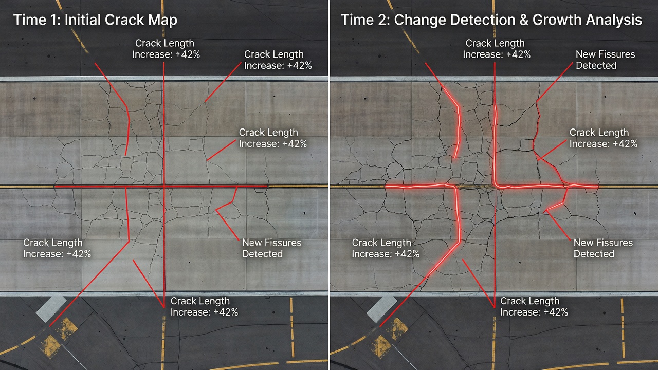
Change detection compares co-registered images or point clouds of the same structure taken at different times to identify new, worsening, or repaired defects — cracks that grew, spalls that enlarged, corrosion that spread. It enables quantitative deterioration tracking over time for infrastructure monitoring.
Change Detection for Infrastructure Monitoring
Definition and Purpose
Change detection is the process of identifying differences in the state of a structure, surface, or environment by comparing observations acquired at different points in time. In the context of civil infrastructure monitoring, change detection systematically compares co-registered images, orthomosaics, or 3D point clouds of the same asset — a runway, bridge deck, roadway, or building — captured during repeat surveys, to identify new defects, quantify the progression of existing deterioration, and verify the effectiveness of maintenance interventions. Unlike a single-point-in-time inspection that captures only a snapshot of current condition, change detection reveals the temporal dimension of deterioration: which cracks are actively growing, which spalled areas are enlarging, where corrosion is spreading, and what deformations are accumulating.
The fundamental purpose of change detection is to transform infrastructure condition data from static snapshots into dynamic temporal records. A single inspection answers the question “what is the current condition?” Change detection answers the more operationally relevant question “how is the condition changing?” This distinction is critical for infrastructure asset management because deterioration is a dynamic process. A crack that has remained stable at 0.3 mm width for three years presents a different maintenance priority than a crack that grew from 0.3 mm to 1.5 mm in the same period, even though both cracks appear identical in a single inspection. Change detection quantifies this rate of deterioration, enabling condition-based maintenance planning, budget forecasting, and risk assessment that are impossible from static inspections alone.
In airport pavement management under ICAO Annex 14 — Aerodromes, Volume I, the aerodrome operator is required to maintain pavements in a condition that prevents damage to aircraft and is free of loose material. While periodic visual inspections satisfy basic compliance, ICAO Doc 9157 (Aerodrome Design Manual, Part 3: Pavements) and the ASTM D5340 standard for Airport Pavement Condition Index (PCI) emphasize the importance of tracking deterioration trends over time. Change detection provides the quantitative foundation for trend analysis, enabling airport operators to identify pavements with accelerating deterioration rates before they reach critical condition states. The methodology directly supports the ICAO Global Air Navigation Plan (GANP) objectives for infrastructure resilience and risk-based maintenance optimization.
The concept of change detection originates from remote sensing and geospatial analysis, where it was developed for land-use change monitoring, deforestation tracking, and urban development analysis using satellite imagery. These foundational methods — image differencing, principal component analysis, and post-classification comparison — have been adapted and extended for infrastructure applications where the scale of change is much smaller (millimeters to centimeters rather than meters to kilometers) and the accuracy requirements are correspondingly higher. Modern infrastructure change detection operates at sub-millimeter sensitivity for crack measurement and sub-centimeter sensitivity for deformation monitoring.
Image Registration — The Prerequisite for Change Detection
Reliable change detection depends fundamentally on the accuracy of image registration — the process of geometrically aligning two or more images of the same scene so that corresponding pixels represent the same physical location on the structure. Without precise registration, any comparison between images will contain spurious change signals at object edges, texture boundaries, and surface features that are simply misaligned rather than physically changed. Registration errors of even one pixel can produce false change artifacts that overwhelm real defect signals, particularly for small defects like cracks that may be only 2-5 pixels wide in typical infrastructure imagery.
The relationship between registration accuracy and minimum detectable change is governed by the signal-to-noise ratio of the detection system. For pixel-based change detection methods, registration errors appear as additive noise in the difference image. Research consistently demonstrates that sub-pixel registration accuracy — typically better than 0.5 pixels root mean square error (RMSE) — is required for reliable detection of small defect changes. At a ground sample distance (GSD) of 1 mm per pixel (typical for precision runway surveys), this corresponds to 0.5 mm geometric alignment tolerance. Achieving this tolerance across repeat surveys conducted months or years apart requires consistent survey methodologies, stable ground control networks, and robust registration algorithms.
Feature-Based Image Registration
Feature-based registration identifies distinctive, repeatable features in both the reference and target images, establishes correspondences between these features, and computes the geometric transformation that maps the target image into the reference image coordinate system. This approach is the most widely used method for infrastructure change detection because it is robust to variations in illumination, moderate differences in viewing angle, and seasonal changes in surface appearance that do not represent structural deterioration.
The registration pipeline begins with feature detection using algorithms designed for repeatability across different imaging conditions. Scale-Invariant Feature Transform (SIFT) remains the most widely used detector for infrastructure registration, identifying keypoints at locations of high spatial gradient that are robust to scale changes and rotation. Speeded-Up Robust Features (SURF) provides faster computation with comparable performance for many applications. For pavement surfaces where texture is relatively uniform, oriented FAST and rotated BRIEF (ORB) features and AKAZE features offer alternatives with different trade-offs between computational efficiency and matching robustness. A typical 20-megapixel orthomosaic of a 500-meter runway section yields 10,000-50,000 detectable features depending on pavement texture, joint spacing, and surface markings.
Feature matching establishes correspondence between detected features in the reference and target images using descriptor vector similarity, typically measured as Euclidean or Hamming distance between descriptor vectors. The initial set of matches inevitably contains outliers — incorrect correspondences arising from repetitive patterns, similar texture patches, or feature ambiguity. Outlier rejection uses RANSAC (Random Sample Consensus) or its variants (MLESAC, MSAC) to iteratively estimate the transformation model while classifying matches as inliers or outliers based on their consistency with the estimated model. A RANSAC threshold of 2-3 pixels at the orthomosaic resolution is typical for infrastructure change detection, rejecting matches whose residual error exceeds this value.
The geometric transformation model is selected based on the expected deformation between surveys. For repeat drone surveys conducted with consistent flight parameters and RTK positioning, a similarity transformation (translation, rotation, uniform scale) or affine transformation (six parameters: two translations, two scales, two shears) is typically sufficient. For surveys with significant perspective differences or terrain variation, a projective transformation (eight parameters, also called homography) or polynomial transformation (higher-order, typically 2nd or 3rd order for large-area surveys) may be required. The transformation is computed from the inlier correspondences using least-squares estimation, with the residual RMSE serving as the primary quality metric. Registration RMSE below 0.5 pixels is the target for high-quality change detection; RMSE above 1 pixel indicates the need for improved control points or transformation model selection.
Intensity-Based Image Registration
Intensity-based registration works directly with pixel intensity values rather than discrete features, optimizing the transformation parameters to maximize a similarity metric computed over the overlapping image region. This approach is advantageous when the image content lacks sufficient distinctive features for reliable feature matching — for example, freshly placed concrete surfaces, uniformly textured asphalt, or surfaces covered with water or debris. Intensity-based methods are also used for fine-tuning after an initial feature-based registration, achieving the sub-pixel accuracy required for high-sensitivity change detection.
The optimization process iteratively transforms the target image, computes the similarity metric against the reference image, and adjusts the transformation parameters to improve the metric. Common similarity metrics include:
Normalized Cross-Correlation (NCC) computes the correlation coefficient between corresponding pixel intensities after normalizing each image window to zero mean and unit standard deviation. NCC values range from -1 to +1, with values close to 1 indicating strong alignment. NCC is robust to linear intensity differences between images, making it suitable for surveys with different exposure settings or minor illumination changes.
Mutual Information (MI) measures the statistical dependence between intensity distributions of the two images, based on information entropy. MI is particularly robust to non-linear intensity differences between images, such as those caused by different sensor types, seasonal vegetation changes, or wet-versus-dry surface conditions. The MI between two perfectly aligned images of the same scene is maximized when the joint intensity distribution has minimum entropy — i.e., the relationship between intensities is as predictable as possible.
Sum of Squared Differences (SSD) and Sum of Absolute Differences (SAD) are the simplest metrics, directly computing the pixel-wise intensity difference. They assume that corresponding pixels in the two images should have identical intensities after geometric alignment, an assumption that is rarely valid in practice due to illumination, exposure, and sensor response variations. SSD and SAD are typically used only for multi-view stereo matching within a single survey epoch, not for cross-temporal change detection.
Optimization algorithms for intensity-based registration include gradient descent, Powell’s method, and the Levenberg-Marquardt algorithm. Multi-resolution (coarse-to-fine) strategies are standard, starting with downsampled images to estimate approximate alignment and progressively refining at higher resolutions. For infrastructure change detection, intensity-based registration typically achieves 0.1-0.3 pixel accuracy after fine-tuning, compared to 0.3-0.8 pixel accuracy for feature-based methods alone.
Geo-Referenced Registration Using GCPs and GNSS
Geo-referenced registration uses surveyed ground control points (GCPs) and precise camera positions from RTK (Real-Time Kinematic) or PPK (Post-Processed Kinematic) GNSS to directly establish the geometric relationship between images and real-world coordinates. Each image is geotagged with its camera position (X, Y, Z) and orientation (omega, phi, kappa) from onboard GNSS/IMU, and this information is refined during photogrammetric processing using GCPs surveyed to centimeter-level accuracy.
For change detection, the key advantage of geo-referenced registration is that repeat surveys are inherently aligned to the same coordinate system, significantly reducing the registration problem. Instead of computing pairwise transformations between survey epochs, each survey is independently processed to produce orthomosaics and point clouds in a common coordinate reference system (typically WGS84 with local transverse Mercator projection). The remaining misalignment between surveys is then corrected using a residual transformation estimated from stable features visible in both datasets — pavement markings, runway lights, joint seals, or dedicated survey targets.
The ISO 19157 standard for geographic information quality specifies positional accuracy requirements for geospatial data, which directly apply to geo-referenced change detection. For infrastructure monitoring, typical accuracy targets are horizontal RMSE better than 3 cm and vertical RMSE better than 5 cm for pavement surveys. When these accuracies are achieved through GCP-based photogrammetry or RTK drone positioning, the residual registration error between repeat surveys is typically 1-3 pixels at 1 mm GSD, which is then further reduced through fine registration to the sub-pixel level.
The ICAO Annex 15 — Aeronautical Information Services establishes quality requirements for aeronautical data that influence change detection survey design. Survey data used for airport pavement management must meet defined accuracy, resolution, and integrity levels commensurate with the criticality of the data. For change detection applications where survey data informs maintenance decisions affecting runway safety, the data quality requirements are correspondingly stringent, requiring documented accuracy verification using independent check points and comprehensive metadata reporting.
Change Detection Methods
Image Differencing
Image differencing is the most direct and computationally efficient change detection method. After registration, the pixel-wise difference between the reference image and the target image is computed: Difference(x, y) = I_target(x, y) - I_reference(x, y). For grayscale images with 8-bit intensity values (0-255), the difference image ranges from -255 to +255, typically rescaled to 0-255 for visualization. Areas of no change produce near-zero difference values (subject to sensor noise and minor illumination variation), while areas of physical change produce significant positive or negative deviations.
The critical parameter in image differencing is the change threshold — the difference magnitude above which a pixel is classified as changed. Selecting an appropriate threshold requires balancing detection rate (correctly identifying true changes) against false alarm rate (incorrectly classifying unchanged pixels as changed). The optimal threshold depends on the signal-to-noise ratio of the imaging system, the registration accuracy, and the magnitude of the changes being targeted. Common approaches for threshold selection include:
Standard deviation thresholding sets the threshold at k × σ, where σ is the standard deviation of the difference image in areas known to be unchanged, and k is a multiplier typically between 2 and 5. A threshold of 3σ corresponds to approximately 99.7% confidence that a pixel difference exceeding this value represents real change, assuming normally distributed noise.
Otsu’s method computes the threshold that minimizes intra-class variance between change and no-change pixels, automatically adapting to the statistical properties of each difference image. This is effective when the change area is a moderate fraction of the total image (5-30%).
Bayesian thresholding models the difference image as a mixture of two distributions — no-change pixels following a narrow Gaussian distribution centered at zero, and change pixels following a broader distribution with possibly non-zero mean. Expectation-Maximization (EM) algorithm estimates the parameters of both distributions, and the optimal threshold is computed from the intersection of the two distributions.
Image differencing is most effective for detecting changes in surface appearance: new cracks (dark linear features on light pavement), staining from leakage or chemical spill, vegetation growth, and surface discoloration from corrosion initiation. It is less effective for quantifying geometric changes that do not produce strong intensity differences — for example, crack widening where the crack was already visible in the reference image and the width increase produces only subtle edge shifts.
Principal Component Analysis (PCA)
Principal Component Analysis (PCA) applied to change detection transforms multi-temporal image data into a new coordinate system where change information is concentrated in specific components. For a pair of images (reference and target), PCA is computed on the combined data matrix, producing two principal components. The first principal component captures the common information — the pixels that are similar between the two images. The second principal component captures the residual difference — the change information.
The advantage of PCA over simple differencing is that it automatically decorrelates the data, separating change signals from systematic differences in overall brightness, contrast, and sensor response. This makes PCA more robust to illumination variations between surveys. The PCA change image (typically the second principal component) often reveals subtle changes that would be buried in noise using direct differencing.
For multi-temporal analysis with three or more survey epochs, Multivariate Alteration Detection (MAD) extends the PCA concept. MAD finds linear transformations of the multi-temporal data that maximize the correlation between transformed bands, then identifies changes as deviations from this correlation structure. The MAD components are ordered by decreasing change information content, enabling the analyst to focus on the most significant change signals. Iteratively Reweighted MAD (IR-MAD) improves robustness by iteratively downweighting pixels identified as changed in previous iterations, refining the no-change background model.
Machine Learning-Based Change Detection
Machine learning methods for change detection have advanced significantly with the availability of large training datasets and deep learning architectures. These methods learn the mapping from image pairs to change maps directly from labeled examples, rather than relying on hand-crafted thresholds or statistical models. Three main categories of ML-based change detection are relevant to infrastructure monitoring:
Pixel-based classification treats each pixel independently, classifying it as change or no-change based on features extracted from the corresponding pixels in both images plus neighborhood context. Features may include spectral differences, texture measures (GLCM, Gabor filters), local spatial statistics, and multi-scale representations. Random Forest, Support Vector Machines (SVM), and Gradient Boosting classifiers are common choices. Training requires labeled change maps for a representative set of infrastructure surfaces and defect types.
Patch-based deep learning uses convolutional neural networks (CNNs) operating on image patches centered at each pixel. A siamese network architecture processes the reference patch and target patch through two identical CNN branches with shared weights, then a comparison module (concatenation, differencing, or correlation) fuses the feature representations, and a classification head produces the change probability for the central pixel. UNet-based architectures with skip connections are particularly effective for change detection because they preserve spatial resolution while integrating multi-scale context. Training datasets for infrastructure change detection must include representative examples of each defect type (cracks, spalls, corrosion, staining) under varying illumination and surface conditions.
Object-based change detection (OBIA) first segments the image into meaningful objects — individual pavement panels, crack segments, spalled regions — then compares objects across time rather than pixels. This approach is particularly well-suited for infrastructure monitoring because defects are naturally object-like: a spall is a contiguous region, a crack is a linear feature, corrosion patches are spatially coherent. Object-based change detection computes changes in object properties (area, perimeter, shape, mean intensity) and classifies objects as stable, growing, shrinking, or new. The object-based approach inherently reduces noise from isolated pixel artifacts and provides change information in terms directly relevant to infrastructure condition assessment — area of new spalling, length of crack extension, percentage increase in corrosion coverage.
Method
Typical Accuracy
Strengths
Limitations
Image Differencing
60-75% pixel accuracy
Simple, fast, interpretable
Sensitive to illumination, needs optimal threshold
PCA / MAD
70-85% pixel accuracy
Robust to brightness variations
Requires multi-spectral or multi-temporal data
Random Forest / SVM
75-88% pixel accuracy
Handles non-linear relationships
Needs labeled training data, limited generalization
CNN (siamese UNet)
85-95% pixel accuracy
High accuracy, learns spatial context
Large training data required, computationally intensive
OBIA
80-92% object accuracy
Change metrics match defect semantics
Segmentation quality dependent, complex workflow
Crack Change Detection
Crack Growth Quantification
Crack change detection is the most common and operationally important application of temporal analysis for infrastructure monitoring. Crack growth — the increase in crack width, length, or density over time — is the primary indicator of active deterioration in concrete and asphalt structures. Change detection for cracks must operate at sub-millimeter sensitivity because the differences being measured are often smaller than the crack itself: a crack that was 0.5 mm wide in the baseline survey and is 1.2 mm wide in the follow-up survey represents a 0.7 mm change that must be reliably detected against image noise and registration uncertainty.
Pixel-level crack change detection uses differential crack mapping, where crack probability maps from each survey epoch are compared. The crack probability map — generated by a deep learning crack segmentation model or by a conventional crack detection algorithm — assigns each pixel a value between 0 (no crack) and 1 (definite crack). The change map is the per-pixel difference in crack probability between epochs, with positive values indicating new or widened cracks and negative values indicating healed or sealed cracks. Morphological filtering removes isolated changed pixels, and connected component analysis groups changed pixels into discrete change objects.
Quantitative crack width change measurement requires sub-pixel edge localization. For each crack segment in the crack network, the crack edges are extracted at sub-pixel resolution using methods such as stepped edge detection (fitting the edge response to a step function and finding the sub-pixel zero-crossing), moment-based edge detection (computing edge position from image moments), or active contour models (snakes) that evolve to match the crack boundaries. The width at each point along the crack is computed as the distance between the two edge sub-pixel positions measured perpendicular to the crack centerline. Width change is then the per-point difference between epochs, and mean width increase over the crack segment length is the summary statistic. For airport pavement surveys at 1 mm GSD, crack width change of 0.2-0.3 mm is reliably detectable using sub-pixel methods with 0.1 pixel edge localization precision.
Crack length extension measures the increase in the total length of the crack network. This requires vectorizing the crack skeleton in each epoch as a set of polylines, then matching crack segments between epochs using spatial overlap and proximity criteria. New crack extension appears as crack segments in the follow-up survey that do not overlap with any crack segment in the baseline survey but are connected to existing cracks. Crack growth rate — mm per month or mm per year — is computed by dividing the total length increase by the time interval between surveys. For highway and airport pavements, typical crack growth rates range from 0.5-5 mm per month depending on traffic loading, environmental conditions, and pavement structural capacity.
New Crack Detection
New crack detection identifies crack pixels or crack objects that appear in the follow-up survey but were absent in the baseline survey. This requires distinguishing actual new cracks from false positives caused by registration misalignment, illumination differences, or surface moisture artifacts. The detection process typically involves the following steps:
Baseline crack mask generation using a validated crack detection model with known false positive rate. The baseline mask should conservatively over-segment rather than under-segment — including uncertain crack candidates reduces the chance of missing new cracks that were partially visible in the baseline survey.
Follow-up crack mask generation using the same crack detection model and processing parameters applied to the co-registered follow-up orthomosaic. Consistent application of the detection algorithm is essential; changes in the detection model or processing parameters between epochs would introduce non-physical change signals.
Change mask computation by identifying pixels that are crack in the follow-up mask but non-crack in the baseline mask. Morphological opening (erosion followed by dilation) removes isolated pixel noise and thin artifacts at crack edges caused by sub-pixel misregistration.
Geometric filtering eliminates change objects that do not satisfy crack geometry criteria — minimum length (typically >10 pixels), minimum aspect ratio (length-to-width ratio >3), and connectivity to existing crack networks. Isolated pixel clusters that do not form linear features are classified as non-crack artifacts.
Validation against manual inspection or ground truth for a sample of detected changes to calibrate the false positive rate and adjust detection parameters.
The minimum detectable new crack width is approximately the GSD of the imagery — typically 1-2 mm for runway surveys. Cracks narrower than the GSD may still be detectable if they produce a measurable intensity difference (contrast) in the image, but the detection confidence decreases for sub-pixel-width cracks. TarmacView’s crack change detection pipeline achieves 90-95% detection rate for new cracks wider than 2 mm at 1 mm GSD, with a false positive rate below 5% for typical airport pavement surfaces.
Spall and Corrosion Change Detection
Spall Area Change
Spalling — the fragmentation and detachment of surface material from concrete or masonry — produces visible depressions, exposed aggregate, and sharp edges at the boundary between sound and deteriorated material. Change detection for spalls quantifies the increase in spall area, depth, and perimeter over time. Unlike crack detection, which operates on linear features, spall detection requires accurate delineation of irregular area features.
Spall change detection uses segmentation-based comparison between survey epochs. The spall boundary in each orthomosaic is delineated either manually by inspectors, semi-automatically using interactive segmentation tools (grab cut, watershed, or active contour algorithms), or fully automatically using deep learning segmentation models (Mask R-CNN, DeepLab, or UNet trained on spall datasets). Once the spall boundaries are extracted as polygons in each epoch, the change metrics are computed:
Area change = Area_followup - Area_baseline (typically reported in cm² or m²). Area growth rate = Area change / time interval (cm²/month or m²/year). Perimeter change measures complexity of the spall boundary as it advances into previously sound material. Radial growth measures the maximum distance from the original spall boundary to the new boundary in any direction, indicating the direction of fastest deterioration.
For concrete structures, spall growth rates vary widely depending on the cause mechanism. Spalls caused by corrosion-induced delamination typically grow at rates of 1-5 cm of radial extension per year in aggressive environments. Spalls caused by freeze-thaw action show seasonal growth patterns concentrated in winter and spring. Spalls caused by impact or overloading are typically sudden in onset and may remain stable if the loading cause is addressed.
Corrosion Spread Mapping
Corrosion change detection identifies areas where corrosion products (rust on steel, oxidation staining on concrete) have appeared, spread, or intensified between survey epochs. Corrosion appears as characteristic discoloration — orange, brown, or red-brown on steel surfaces; rust-colored staining on concrete surfaces — that is detectable in visible-spectrum imagery. The spectral signature of corrosion is distinct from most other surface features, enabling relatively robust detection.
Corrosion index computation converts RGB imagery to a corrosion-sensitive metric. Common indices include: the Red/Green ratio (corroded areas have higher red reflectance relative to green); the Normalized Corrosion Index NCI = (Red - Green) / (Red + Green); and the Rust Index RI = (2 × Red - Green - Blue) normalized by intensity. These indices are thresholded to produce binary corrosion maps in each epoch.
Corrosion coverage change is the percentage increase in corrosion-affected area relative to the total surface area. For steel bridges and components, the change detection threshold is typically 1-2% of total surface area for significant corrosion progression. For concrete surfaces with staining, smaller area thresholds are used (0.5-1%) because staining is often more spatially distributed than pitting corrosion on steel.
Corrosion severity change categorizes corrosion progression by severity level following standards such as ISO 4628-3 (Paints and varnishes — Evaluation of degradation of coatings — Part 3: Degree of rusting) or SSPC-VIS 2 (Standard for evaluating degree of rusting on painted steel surfaces). Change detection assigns a severity level to each corrosion patch in each epoch and flags patches that have advanced to a higher severity level between surveys. Severity levels are based on the percentage of visible surface area affected by rust: Ri0 (0%), Ri1 (<0.05%), Ri2 (0.05-0.5%), Ri3 (0.5-1%), Ri4 (1-5%), Ri5 (>5%) per ISO 4628-3.
Point Cloud Change Detection
Cloud-to-Cloud (C2C) Comparison
Cloud-to-Cloud (C2C) distance is the simplest method for comparing two point clouds. For each point in the reference cloud, the nearest neighbor in the target cloud is found, and the Euclidean distance between them is computed. The result is a per-point distance value that can be visualized as a color-coded distance map, with blue indicating no change (near-zero distance) and red indicating large change.
The advantages of C2C are computational efficiency (O(n log n) with kd-tree acceleration) and conceptual simplicity. However, C2C has fundamental limitations for infrastructure change detection. First, it measures the shortest distance to any point in the target cloud, not the distance in the surface-normal direction, which can significantly underestimate deformation magnitude on inclined surfaces. Second, C2C is sensitive to point density variations between clouds — a higher density cloud will systematically show smaller nearest-neighbor distances regardless of physical change. Third, C2C provides no confidence interval for the distance measurement, making it difficult to distinguish real deformation from measurement noise.
For these reasons, C2C is best used as a rapid screening method to identify regions of potential change, followed by more rigorous analysis of those regions using more sophisticated methods. In practice, C2C with a threshold of 2-3 times the point cloud noise level provides a conservative change detection screen that captures most significant changes while minimizing false positives from noise and density variation.
Multiscale Model-to-Model Cloud Comparison (M3C2)
M3C2 is the current state-of-the-art algorithm for point cloud change detection, developed by Lague, Brodu, and Leroux (2013) and widely adopted in geomorphology and infrastructure monitoring. M3C2 addresses the limitations of C2C by computing distances along the local surface normal direction at a scale appropriate to the surface roughness, with statistically rigorous confidence intervals.
The M3C2 algorithm operates as follows:
Normal vector computation at each point in the reference cloud by fitting a plane to the local neighborhood. The neighborhood radius (D/2) is chosen to match the scale of surface features being analyzed — smaller radii for fine-scale features like cracks, larger radii for broad deformation patterns. For infrastructure monitoring, typical radii range from 10 cm for detailed crack analysis to 1 m for overall deformation assessment.
Projection and distance computation along the normal direction. For each point in the reference cloud, a cylinder of radius d (projection scale) is oriented along the normal vector. Points from both the reference and target clouds that fall within this cylinder are identified. The distance between the two point sets along the normal direction is computed as the difference between their mean positions along the normal vector. The projection scale d is typically set to 2-5 times the mean point spacing to ensure sufficient points for robust mean computation.
Confidence interval estimation using the local point cloud roughness and point count. The M3C2 algorithm computes a 95% confidence interval (or any specified confidence level) for the distance measurement at each point, based on the standard deviation of points within the projection cylinder and the number of points. Changes smaller than the confidence interval are not statistically significant and should not be interpreted as real deformation. This built-in statistical quality control is the key advantage of M3C2 over simpler methods.
Multi-scale analysis allows the operator to analyze changes at multiple spatial scales simultaneously. Fine-scale analysis (small D/2 and d) detects small features like crack opening and spall boundaries. Coarse-scale analysis (large D/2 and d) detects broad deformation like bridge deflection and differential settlement. Comparing results across scales can distinguish surface change (erosion, deposition, spalling) from deformation (structural displacement, tilt, settlement).
For infrastructure monitoring, M3C2 achieves detection sensitivity of 0.5-2 mm for terrestrial laser scanner point clouds with densities exceeding 500 points/m². For photogrammetric point clouds (which typically have more noise than TLS data), detection sensitivity is 2-5 mm depending on surface texture, image quality, and survey geometry. The algorithm is implemented in the open-source software CloudCompare and is the standard method for point cloud change detection in infrastructure applications worldwide.
DOD compares Digital Elevation Models (DEMs) or Digital Surface Models (DSMs) generated from point clouds in each survey epoch. The two DEMs are subtracted to produce a difference raster where each pixel value represents the elevation change at that location. DOD is computationally efficient because it operates on regular grids rather than unstructured point clouds, and the results are easy to visualize and interpret as heat maps of elevation change.
The accuracy of DOD depends on the DEM generation quality — interpolation from irregular point clouds to regular grids introduces additional uncertainty. The Level of Detection (LoD) for DOD is computed as LoD = t × √(σ_baseline² + σ_followup²), where σ is the elevation uncertainty of each DEM and t is the Student’s t value for the desired confidence level (typically t = 1.96 for 95% confidence). DOD is most appropriate for monitoring bulk volume changes — material loss from erosion or spalling, material accumulation from sediment or debris, and large-scale settlement or heave. It is less suitable for fine-scale defect detection where individual crack or spall details are needed.
Repeat Drone Survey Cadence
Survey Frequency Determination
The optimal interval between repeat surveys for change detection depends on the rate of deterioration, the criticality of the asset, regulatory requirements, and the minimum detectable change of the measurement system. The fundamental principle is that the survey interval should be short enough that the expected deterioration over the interval exceeds the detection threshold of the change analysis, but long enough that the cumulative changes are operationally meaningful and economically justified.
For airport pavements under ICAO Annex 14 compliance frameworks, the typical survey cadence is:
Annual surveys for all operational pavements (runways, taxiways, aprons) as part of routine condition monitoring. Annual surveys establish the baseline deterioration rate and identify areas requiring more frequent attention. ICAO Annex 14, Section 10.2 requires that “the surface of pavements shall be inspected at regular intervals” and that “the frequency of inspections shall be determined by the type and volume of traffic and the prevailing climatic conditions.”
Quarterly surveys for pavements in poor condition (PCI < 40) or with known active deterioration. Quarterly change detection tracks the effectiveness of interim maintenance and provides early warning of rapid deterioration that may require structural intervention.
Monthly surveys for pavements under observation for critical defects — cracks near pavement edges that could lead to spalling, areas of active settlement, or pavement sections subject to high-stress operations (e.g., runway ends where aircraft turn and apply high torque).
Post-event surveys after extreme weather events (heavy rainfall, freeze-thaw cycles, extreme heat), after unusual loading events (overweight aircraft, hard landings), or after maintenance interventions to verify effectiveness.
For bridge structures, inspection intervals are governed by national bridge inspection standards (e.g., NBIS in the United States, DIN 1076 in Germany, BASt guidelines in Europe). Routine visual inspections are typically biennial, but change detection surveys for known defects may be conducted at different frequencies:
Biennial surveys for bridges in good condition with no known significant defects. These establish baseline deterioration rates for comparison with future surveys.
Annual surveys for bridges with known defects under observation — cracks in critical members, corrosion in steel components, scour vulnerability, or movement at bearings.
Quarterly to semi-annual surveys for bridges with active deterioration being monitored for rate of progression, post-repair verification, or bridges with remaining service life under 5 years.
Data Consistency Requirements
Reliable change detection across repeat surveys requires careful control of data collection parameters to minimize non-physical differences between epochs. Key consistency requirements include:
Ground Sample Distance (GSD) should be consistent across surveys within 10-20%. Significant changes in GSD alter the spatial resolution at which defects are measured and can introduce apparent changes that are purely artifacts of resolution differences. GSD consistency is achieved by flying at the same altitude with the same camera sensor across all survey epochs.
Illumination conditions should be as consistent as possible. Surveys conducted in direct sunlight produce strong shadows from cracks and surface texture that differ from surveys in overcast lighting. The recommended practice is to conduct all repeat surveys under similar lighting conditions — preferably overcast with diffuse illumination, which minimizes shadows and provides the most uniform surface appearance for defect detection.
Surface moisture should be consistent. Wet pavement surfaces appear significantly different from dry pavement — cracks fill with water and become less visible, surface staining appears darker, and overall reflectance decreases. Surveys should be conducted only when the pavement surface is dry (minimum 48 hours since last rainfall for concrete, 24 hours for asphalt).
Camera and sensor parameters — exposure time, aperture, ISO, focus distance — should be consistent. Automated exposure settings (auto-exposure, auto-ISO) should be disabled in favor of fixed settings determined during survey planning to ensure consistent image radiometry across epochs.
Flight path and overlap should follow the same mission plan across all survey epochs. Using pre-programmed flight plans with the same waypoints, altitude, speed, and overlap settings ensures consistent viewing geometry, which simplifies registration and reduces geometric differences between surveys.
Change Detection Alerts
Alert Threshold Configuration
Change detection alerts translate quantitative change measurements into actionable notifications for infrastructure managers. Alert thresholds define the magnitude of change that triggers a notification, categorized by severity level to support appropriate response prioritization. The configuration of thresholds depends on the defect type, the criticality of the asset, and the operational context.
For crack growth alerts, thresholds are typically based on crack width increase:
Watch level — crack width increase of 0.3-0.5 mm between surveys. Indicates possible active cracking. No immediate action required but increased monitoring frequency recommended. Verification by ground inspection during next scheduled visit.
Warning level — crack width increase of 0.5-1.5 mm between surveys. Indicates confirmed active cracking. Engineering evaluation recommended to determine cause and assess structural implications. Schedule detailed inspection within 30-60 days.
Alarm level — crack width increase exceeding 1.5 mm between surveys (or any single crack width exceeding 5 mm, per ASTM D5340 severity guidelines). Indicates rapidly progressing deterioration. Immediate engineering evaluation required. Restrict loading if crack is in a critical structural element. Schedule repair within 30 days.
For spall growth alerts, thresholds are based on area increase:
Watch level — spall area increase of 10-25% relative to baseline. Monitor at next survey cycle.
Warning level — spall area increase of 25-50% or spall depth increasing beyond the cover depth. Schedule detailed assessment. Evaluate for loose material that could become FOD (Foreign Object Debris) for airfield pavements.
Alarm level — spall area increase exceeding 50% relative to baseline, or any new spall exceeding 25 cm in maximum dimension on airfield pavements (per ICAO Foreign Object Debris guidelines). Immediate ground inspection required. Remove loose material. Schedule repair within 7-14 days.
For corrosion spread alerts, thresholds are based on coverage and severity category change:
Watch level — corrosion coverage increase of 5-15% of the affected area, or progression from Ri2 to Ri3 per ISO 4628-3. Monitor at next survey.
Warning level — corrosion coverage increase of 15-30% or progression from Ri3 to Ri4. Engineering evaluation for coating condition and substrate integrity. Plan recoating within 6-12 months.
Alarm level — corrosion coverage exceeding 30% or progression to Ri5. Immediate evaluation of structural capacity. For steel bridge members, section loss assessment using ultrasonic thickness measurement. Plan intervention within 1-3 months.
Multi-Level Alerting Framework
Effective change detection alerting operates at multiple cascading levels to avoid overwhelming infrastructure managers with notifications while ensuring critical changes are not missed:
Level 1 — Statistical Alert triggers when the change magnitude exceeds a statistical threshold derived from the measurement noise. This is the lowest-level alert, indicating that the observed change is statistically significant (exceeds the 95% confidence interval of the measurement system). Many level 1 alerts are expected during routine monitoring and do not require immediate attention.
Level 2 — Operational Alert triggers when the change magnitude exceeds a predefined threshold that experience has shown indicates active deterioration requiring attention. Operational alerts are specific to each asset and defect type, calibrated based on historical deterioration data and maintenance records.
Level 3 — Critical Alert triggers when the change magnitude indicates an immediate safety concern — rapid crack growth in a critical structural member, sudden settlement of a bridge abutment, or spall development that could generate FOD on an active runway. Critical alerts require immediate notification of responsible personnel and expedited response within hours to days.
The alert framework should also incorporate temporal consistency — changes that persist or grow across multiple survey epochs receive higher priority than isolated changes that do not progress. A crack that shows 0.4 mm growth in one survey interval but stabilizes in the next should be downgraded from Warning to Watch, while a crack that shows consistent 0.3-0.5 mm growth in each of three consecutive surveys should be escalated.
Integration with Deterioration Models
From Change Detection to Deterioration Prediction
Change detection data provides the empirical foundation for deterioration models that predict future condition states and remaining service life. The integration of change detection with deterioration modeling transforms reactive maintenance — fixing defects when they reach critical condition — into proactive, condition-based maintenance planning where interventions are scheduled based on predicted deterioration trajectories.
Empirical deterioration curves are developed by plotting change detection results over multiple survey epochs. For each defect type and structural element, the change rate (crack width growth in mm/year, spall area growth in cm²/year, corrosion coverage increase in %/year) is computed from the time series of survey measurements. These empirical rates are then used to project future condition states assuming continued deterioration at the observed rate. For airport pavements, the Pavement Condition Index (PCI) deterioration curve is typically modeled as an exponential decay: PCI(t) = PCI_initial × exp(-k × t), where k is the deterioration rate constant derived from change detection measurements across multiple survey cycles.
Probabilistic deterioration models incorporate the uncertainty in both measurement and prediction. Change detection provides not only the change magnitude but also the confidence interval for that measurement (from M3C2 or from statistical change analysis). These uncertainties propagate into the deterioration model, producing confidence bounds on predicted future condition. A Markov chain model, for example, uses the change detection data to estimate transition probabilities between condition states, with confidence intervals reflecting the measurement uncertainty at each epoch.
Machine learning deterioration prediction uses the temporal sequence of change detection measurements as features for predicting future condition. Recurrent neural networks (RNNs) and Long Short-Term Memory (LSTM) networks are particularly suited to this task because they learn temporal patterns directly from the sequence of survey measurements. Input features include crack width time series, spall area time series, PCI values, and environmental covariates (temperature cycles, precipitation, freeze-thaw events). The model outputs are predicted condition at future time points with associated prediction intervals.
Feedback Loop With Maintenance Actions
Change detection also enables quantitative assessment of maintenance effectiveness through before-and-after comparison. When a defect is repaired — crack sealed, spall patched, corrosion treated — the change detection analysis between the pre-repair survey and the first post-repair survey verifies that the defect is no longer present. Subsequent surveys track whether the repair remains effective or if the defect recurs.
Repair durability tracking over multiple survey cycles provides data on the mean time to re-appearance of defects after different repair methods. This data informs maintenance planning by identifying the most durable repair strategies for each defect type under specific environmental and loading conditions. For example, if change detection reveals that crack sealing on a particular runway section has a median recurrence time of 18 months while routing and sealing has a median recurrence time of 36 months, the higher initial cost of routing and sealing is justified by the extended service life.
Performance-based maintenance contracting uses change detection data to verify that maintenance contractors have achieved specified performance outcomes. A contract may specify that crack width in treated areas must not exceed 125% of the post-repair width for at least 24 months. Change detection surveys at 6, 12, and 24 months post-repair provide objective verification of compliance, with payment tied to demonstrated performance rather than simply completion of work.
Software and Automation for Change Detection
Commercial and Open-Source Tools
CloudCompare is the primary open-source software for point cloud change detection, implementing M3C2, C2C, C2M (Cloud-to-Mesh), and DOD methods. It supports LAS, LAZ, PLY, and other common point cloud formats, provides batch processing for automated pipelines, and includes visualization tools for color-coded change maps. CloudCompare runs on Windows, macOS, and Linux and is the de facto standard for point cloud change analysis in infrastructure monitoring.
Agisoft Metashape supports orthomosaic and DEM comparison for change detection through its workflow for difference computation between processed projects. The software provides automated image registration across surveys using the common GCP network, and the resulting orthomosaics can be compared pixel-wise or through the built-in DEM differencing tool. Metashape’s Python API enables scripting of change detection workflows for batch processing of multiple survey pairs.
Pix4Dmapper and Pix4Dmatic include orthomosaic and DSM comparison capabilities, with automated change detection reports that highlight areas of significant elevation difference. Pix4D’s quality report includes per-pixel accuracy estimates that inform the statistical significance of detected changes.
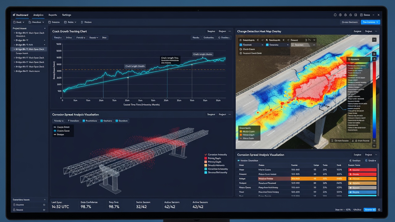
TarmacView provides specialized change detection for airport pavement infrastructure, comparing orthomosaics and crack maps across repeat surveys with automated change classification. The platform tracks crack growth (width and length), new crack formation, spall area changes, and PCI deterioration trends. Change detection results are visualized as overlay maps on the current orthomosaic, with color-coded change severity and automated alert generation for changes exceeding configurable thresholds.
Automated Processing Pipelines
Full automation of change detection requires an integrated pipeline that handles all processing steps from data ingestion to report generation:
Step 1 — Data Ingestion: Import new survey data (images, GNSS logs, GCP coordinates) and retrieve corresponding baseline survey data from the asset database. Validate that both surveys cover the same asset area and meet quality requirements.
Step 2 — Registration: Perform automated registration of the new orthomosaic or point cloud to the baseline reference. For orthomosaics, use feature-based registration with SIFT or AKAZE features followed by intensity-based fine registration. For point clouds, apply coarse registration using GCPs or ICP (Iterative Closest Point) followed by fine registration.
Step 3 — Change Computation: Apply the selected change detection method — image differencing for intensity changes, M3C2 for point cloud deformation, object-based comparison for crack and spall changes. Compute change statistics with confidence intervals.
Step 4 — Classification: Classify detected changes by type (crack growth, new crack, spall spread, corrosion, deformation), severity level, and spatial location. Assign each change object to its corresponding asset component.
Step 5 — Alert Generation: Compare change magnitudes against configured thresholds for each defect type and location. Generate level-1, level-2, or level-3 alerts as appropriate. Record alerts in the asset management system with spatial reference, change magnitude, confidence interval, and time stamp.
Step 6 — Report Generation: Produce change detection reports that include change maps (overlay on current orthomosaic), summary statistics (total crack length change, new defect count, PCI trend), detailed per-defect change data (crack width history, spall area history), and recommended actions based on alert levels.
Step 7 — Database Update: Update the asset condition database with new change detection results. Append time series data for each defect and asset element. Update deterioration curves with the new measurement point. Re-compute predicted condition and remaining service life if deterioration models are integrated.
Quality Assurance for Automated Change Detection
Automated change detection requires systematic quality assurance to ensure that the reported changes are real and not artifacts of processing errors:
Registration quality check: The registration RMSE between surveys must be below the project threshold (typically 0.5 pixels for orthomosaics, 0.5 cm for point clouds). If registration quality is insufficient, the change detection results are flagged for manual review.
False positive screening: Change detection results are screened against known non-change indicators: areas of standing water (detected by near-infrared or thermal imagery), areas of recent maintenance (recorded in the asset management system), and areas with known surface contamination (oil spills, rubber buildup on runways).
Temporal consistency check: Changes that appear in a single survey interval but are not confirmed in subsequent surveys are flagged as potentially transient — surface stains that wash away, moisture patterns that vary with weather, or debris that is removed. Persistent changes receive higher confidence ratings.
Manual review sample: A statistically valid sample of detected changes is reviewed by a qualified inspector for each survey cycle. The sample size is calculated to achieve 95% confidence that the false positive rate of the automated system is below the acceptable threshold (typically 5-10% for watch-level alerts, 1-2% for alarm-level alerts).
Conclusion
Change detection transforms infrastructure inspection from a static condition snapshot into a dynamic temporal record of deterioration, repair, and structural behavior. By precisely co-registering images and point clouds from repeat surveys, change detection quantifies the subtle, millimeter-scale progression of cracks, spalls, corrosion, and deformation that would be invisible in a single inspection but, accumulated over time, determines the service life of the asset.
The methodology integrates rigorous geometric registration — feature-based, intensity-based, or geo-referenced using GCPs — with statistical change analysis that separates real deterioration from measurement noise. The selection of change detection method depends on the defect type and required sensitivity: image differencing for surface appearance changes, M3C2 for point cloud deformation, object-based comparison for crack and spall geometry changes, and machine learning methods for automated classification with high accuracy.
For airport pavements, bridges, and critical infrastructure, change detection provides the data foundation for condition-based maintenance, deterioration modeling, and risk-informed budget allocation. It enables infrastructure managers to identify accelerating deterioration before it reaches critical levels, verify the effectiveness of maintenance interventions, and optimize the timing and scope of repair activities. The integration of change detection with automated processing pipelines, alert frameworks, and deterioration models creates a closed-loop condition management system that continuously improves maintenance decision quality through empirical evidence of deterioration rates and repair durability.
TarmacView implements change detection as a core capability of its airport pavement inspection platform, enabling automated tracking of crack growth, spall spread, and condition trends across successive drone surveys. The platform applies rigorous registration and statistical quality control to ensure that reported changes are real and actionable, providing infrastructure managers with quantitative evidence for maintenance planning and compliance reporting under ICAO Annex 14 and ASTM D5340 standards.
Frequently Asked Questions
Change detection is a temporal analysis technique that compares co-registered images, orthomosaics, or point clouds of the same infrastructure asset captured at different times. It identifies and quantifies differences such as new cracks, crack growth, spall enlargement, corrosion spread, surface deformation, and settlement. The process requires precise image registration or point cloud alignment so that only real physical changes — not misalignment artifacts — appear in the difference analysis.
For pixel-level change detection, registration accuracy should be sub-pixel — typically better than 0.5 pixels RMSE. At a ground sample distance (GSD) of 1 mm/pixel, this translates to 0.5 mm registration accuracy. Registration errors larger than 1 pixel produce false change signals at edges and texture boundaries that can overwhelm real defect changes. Feature-based registration using scale-invariant features and RANSAC outlier rejection routinely achieves 0.3-0.8 pixel accuracy. RTK/PPK geotagging combined with GCPs enables consistent sub-pixel registration across repeat surveys.
Crack change detection typically combines pixel-level and object-level analysis. Pixel-level methods detect changes in crack pixel density within local neighborhoods between time steps. Object-level methods first vectorize cracks in each survey epoch, then compare crack maps by computing width changes at matched locations, length extension of existing cracks, and density of new crack formation. The Lie-group-based Temporal Crack Change Detection (LTCCD) module and PDE-guided methods are advanced approaches that track crack evolution with sub-pixel precision by modeling crack boundaries as propagating fronts.
Multiscale Model-to-Model Cloud Comparison (M3C2) is a statistically rigorous algorithm for computing distances between two point clouds. Unlike simple nearest-neighbor methods, M3C2 computes distances along the local surface normal direction at multiple scales, providing confidence intervals for each distance measurement. It accounts for point cloud roughness, density variation, and registration uncertainty. M3C2 is the standard method for deformation monitoring from repeat LiDAR or photogrammetric surveys, achieving sub-millimeter sensitivity when point cloud density exceeds 500 points/m².
Survey cadence depends on deterioration rate, asset criticality, and regulatory requirements. For airport pavements under ICAO Annex 14, visual inspections are typically annual, but change detection surveys for active deterioration zones may be quarterly or monthly. Bridge decks with known cracking may be surveyed every 6 months during active deterioration and every 2-3 years for routine condition tracking. The minimum detectable change is approximately 2.5-3 times the survey accuracy (95% confidence), so survey frequency should be calibrated so that the expected deterioration over the interval exceeds the detection threshold.
Change detection alerting uses multi-level thresholds: (1) pixel-level change magnitude thresholds to filter noise; (2) spatial clustering minimum area thresholds to eliminate isolated pixel artifacts; (3) temporal consistency checks requiring changes to persist or grow across multiple surveys; and (4) severity classification (e.g., crack width increase >0.5 mm triggers watch, >1.5 mm triggers alarm). Alerts are typically configured per defect type — crack growth alerts use width increase thresholds, spall alerts use area increase thresholds, and deformation alerts use displacement magnitude thresholds.
Yes. Change detection workflows typically classify detected changes into three categories: (1) new defects — areas that were classified as sound in the baseline survey but show crack or spall pixels in the follow-up survey; (2) worsening defects — existing cracks that have increased in width, length, or density; and (3) repaired defects — areas where previously identified defects are no longer present after maintenance. This classification requires precise co-registration of defect maps across survey epochs, typically using vectorized crack networks or pixel-wise defect labels with temporal correspondence.
Several platforms support infrastructure change detection: CloudCompare (open-source) implements M3C2, C2C, and C2M algorithms for point cloud comparison; Metashape and Pix4D support orthomosaic comparison and DSM differencing; Cyclone Register 3D and FARUS Scene handle LiDAR time-series analysis. TarmacView provides specialized change detection for airport pavements, comparing orthomosaics and crack maps across repeat surveys with automated change classification, crack growth measurement, and trend analysis per ASTM D5340 and ICAO guidelines.
Automated Change Detection for Infrastructure
TarmacView enables automated change detection across repeat drone surveys of airport pavements, bridges, and infrastructure. Track crack growth, spall enlargement, and deterioration trends with quantitative precision. Identify changes early and optimize maintenance planning.
A point cloud is a set of 3D data points representing the external surfaces of objects or terrain, generated by LiDAR scanning or photogrammetry. In infrastruct...
Semantic Segmentation for Infrastructure Scene Understanding
Semantic segmentation assigns a category label to every pixel in an image, enabling full-scene understanding for infrastructure inspection. Covers encoder-decod...
37 min read
Technology
Computer Vision
+3
Cookie Consent We use cookies to enhance your browsing experience and analyze our traffic. See our privacy policy.