Pixel-Level Crack Segmentation for Infrastructure Inspection

1. Definition and Difference from Crack Classification

Crack segmentation is a dense pixel prediction task within computer vision that assigns a binary label (crack or non-crack) to every individual pixel in an input image. The output is a binary segmentation mask of the same spatial dimensions as the input, where crack pixels are marked as foreground (typically white or value 1) and non-crack pixels as background (black or value 0). This mask preserves the exact morphology, topology, and geometry of every crack present in the scene, including branches, isolated fragments, and sub-millimeter-width fissures.

Crack classification operates at the image level — the model outputs a single scalar indicating whether a crack is present anywhere in the image. A classification model might predict “crack present: 93% confidence” but cannot localize where the crack is, how long it is, or how wide it has grown. This is fundamentally insufficient for infrastructure inspection where precise measurements drive maintenance prioritization, repair cost estimation, and structural safety assessment.

Crack detection via object detection (Faster R-CNN, YOLO, SSD) outputs bounding boxes around crack regions. While detection provides localization, a bounding box around a thin, elongated crack contains mostly background pixels and conveys no information about crack width, topology, or branching structure. A crack that serpentines across a runway may require dozens of overlapping bounding boxes with no semantic relationship between them.

Crack segmentation solves all these limitations. Every crack pixel is identified, enabling direct measurement of:

• Crack area in square millimeters (pixel count × spatial resolution)
• Crack length along the skeletonized centerline in millimeters
• Crack width (mean, maximum, and per-pixel width profiles)
• Branching patterns (number of branches, junction points, fractal dimension)
• Component statistics (total number of distinct cracks, spatial density, connectivity)

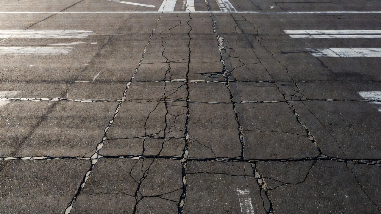
The International Civil Aviation Organization (ICAO) Annex 14 — Aerodromes, Volume I, specifies that runway surfaces must be regularly inspected for deterioration including cracking. ICAO Doc 9157, Part 3 — Pavements, provides guidance on pavement evaluation methods. Traditional manual inspection involves inspectors walking the runway, marking cracks with chalk or spray paint, and recording observations on paper forms — a process that is subjective, inconsistent, hazardous (exposure to live airside operations), and impossible to perform at sub-millimeter precision. Automated crack segmentation replaces subjective visual estimation with reproducible, quantitative, pixel-accurate measurements that can be compared across inspections and across airports.

The transition from classification to segmentation represents a fundamental leap in capability. Classification answers “is there a crack here?” Segmentation answers “exactly where is every crack, how large is it, what shape does it have, and how severe is the damage?” For TarmacView’s crack_seg_head, this dense pixel prediction capability is the foundation for producing high-accuracy crack masks that feed directly into pavement condition index calculations, repair quantity estimation, and longitudinal trend analysis.

2. Segmentation Architectures

U-Net

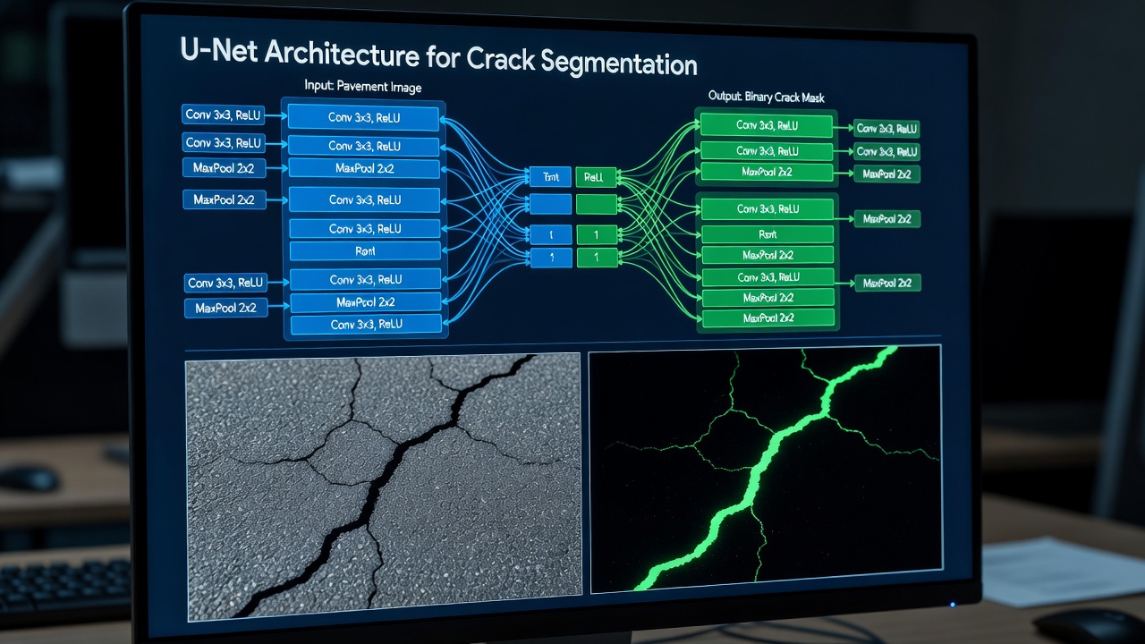
The U-Net architecture, introduced by Ronneberger, Fischer, and Brox in 2015 for biomedical image segmentation, has become the most widely adopted architecture for crack segmentation in infrastructure applications. U-Net consists of a symmetric encoder-decoder structure with four or five resolution levels connected by skip connections that transmit high-resolution spatial information directly from encoder to decoder layers.

The encoder (contracting path) applies repeated 3×3 convolutions followed by ReLU activation and 2×2 max pooling, progressively reducing spatial dimensions while increasing feature channel depth from 64 to 512 or 1024 channels. Each encoder block learns increasingly abstract representations — from simple edge detectors in the first layer to complex crack texture and morphology detectors in the deepest layers. For crack segmentation, the encoder must learn to distinguish true crack features from crack-like textures including aggregate shadows, tire marks, construction joints, surface debris, and sealant streaks.

The decoder (expanding path) performs the mirror operation: 2×2 up-convolution (transposed convolution) doubles spatial resolution while halving channel depth, then concatenates the corresponding encoder feature map via the skip connection, followed by two 3×3 convolutions with ReLU. The final layer uses a 1×1 convolution with sigmoid activation to produce the binary crack mask.

Skip connections are the critical innovation in U-Net. In standard encoder-decoder architectures, all spatial detail is lost during downsampling and must be re-learned in the decoder. Skip connections directly transfer fine-grained spatial information — crack edges, thin crack lines, and precise boundaries — from encoder to decoder at each resolution level. This is essential for crack segmentation because cracks are inherently thin structures (often 1-10 pixels wide) that would be completely lost at the bottleneck level (32× downsampled).

For crack segmentation specifically, U-Net variants include:

• Attention U-Net: Adds attention gates that suppress irrelevant background features while emphasizing crack regions
• Residual U-Net: Replaces standard convolutions with residual blocks, enabling deeper networks without vanishing gradients
• Dense U-Net: Uses dense blocks (DenseNet-style) for improved feature propagation and gradient flow
• U-Net++ : Adds nested skip connections with dense convolutional blocks, reducing the semantic gap between encoder and decoder features

U-Net achieves state-of-the-art performance on crack segmentation benchmarks including CRACK500 (IoU 0.65-0.72) and DeepCrack (IoU 0.70-0.78) when trained with appropriate loss functions and data augmentation.

DeepLabV3+

DeepLabV3+, developed by Google Research (Chen et al., 2018), extends the DeepLab family with an encoder-decoder structure augmented by Atrous Spatial Pyramid Pooling (ASPP) . The core innovation is the use of atrous (dilated) convolutions with multiple dilation rates applied in parallel to capture multi-scale contextual information without reducing spatial resolution.

ASPP applies 3×3 convolutions at different dilation rates — typically rates of 6, 12, and 18 for an output stride of 16 — plus a 1×1 convolution and global average pooling. Each dilation rate captures crack features at a different scale: rate 6 captures fine, narrow cracks (1-3 pixels wide), rate 12 captures medium cracks, and rate 18 captures wide cracks and crack networks. The parallel branches are concatenated and processed by a 1×1 convolution to produce the multi-scale feature representation.

For crack segmentation, DeepLabV3+ excels at handling the extreme scale variation in crack appearance. A single runway image may contain hairline cracks (0.5 mm wide, 1-2 pixels) alongside wide, spalled cracks (15+ mm wide, 30+ pixels). The ASPP module processes all these scales simultaneously. The decoder module upsamples the ASPP features by a factor of 4, concatenates with encoder features from an intermediate layer (before the first atrous block), and applies two 3×3 convolutions followed by bilinear upsampling to the original resolution.

DeepLabV3+ backbones commonly used for crack segmentation include ResNet-50, ResNet-101, and Xception. More recently, EfficientNet and ConvNeXt backbones have been explored, offering improved accuracy-to-parameter ratios. DeepLabV3+ with ResNet-101 backbone achieves IoU scores of 0.68-0.75 on CRACK500 when trained on pavement-specific datasets.

SegFormer

SegFormer (Xie et al., 2021) introduces a hierarchical Transformer encoder with a lightweight MLP (multi-layer perceptron) decoder, representing a departure from CNN-based segmentation architectures. The encoder uses a series of Mix Transformer (MiT) blocks with progressively decreasing resolution (from 1/4 to 1/32 of input size) and increasing channel dimensions. Each MiT block uses efficient self-attention with a reduced spatial reduction ratio, making it computationally feasible for high-resolution crack images.

The key advantage of SegFormer for crack segmentation is the transformer’s global receptive field from the first layer. Unlike CNNs where each layer only sees a local neighborhood (e.g., 3×3 convolution = 1 pixel neighborhood after one layer), Transformers compute attention across the entire feature map. This enables SegFormer to capture long-range dependencies — a crack that snakes across an entire 1024×1024 tile maintains pixel-to-pixel relationships through the attention mechanism.

The MLP decoder in SegFormer is remarkably simple compared to U-Net or DeepLabV3+ decoders. It aggregates multi-level features from all four encoder stages (by upsampling to 1/4 resolution and concatenating), applies a single MLP layer for feature mixing, then another MLP to produce the final segmentation. Despite its simplicity, the MLP decoder achieves strong performance because the hierarchical Transformer encoder already produces well-structured features.

SegFormer-B3 achieves competitive IoU (0.66-0.74) on crack segmentation datasets while being more parameter-efficient than DeepLabV3+ with ResNet-101. The B0-B5 model family provides a trade-off between speed and accuracy, with B0 suitable for real-time edge deployment and B5 for maximum accuracy on server-class hardware.

DINOv2 and DINOv3 Dense Prediction Heads

DINOv2 (Oquab et al., 2023) and DINOv3 represent the latest generation of Vision Transformer (ViT) models trained via self-supervised learning on curated image datasets. Unlike supervised pretraining on ImageNet-1K, DINO uses a self-distillation approach where a student network learns to match the output of a teacher network operating on different views of the same image (local cropped views vs. global views).

The breakthrough of DINO for segmentation is that the self-supervised ViT features — particularly the key (K) and value (V) attention heads in the last layers — naturally encode object boundaries and fine-grained semantic information without any supervised segmentation training. A sparse set of patch tokens (e.g., 0.05% of patches) can be linearly probed to produce segmentation maps that rival fully supervised models.

For crack segmentation, a dense prediction head is attached to the DINO backbone. The typical approach extracts multi-scale features from the last 4-6 layers of the ViT, concatenates them, and applies a convolutional decoder that upsamples to the original image resolution. The decoder may be:

• A lightweight Linear Head: Simply a 1×1 convolution after upsampling the ViT patch tokens (patch size 14×14 for ViT-L/14)
• A Feature Pyramid Network (FPN) head: Multi-scale feature extraction with lateral connections and top-down pathway
• A MaskFormer-style head: Transformer decoder that cross-attends to DINO features and produces binary masks

DINOv3-based crack segmentation achieves IoU scores exceeding 0.78 on CRACK500 and 0.82 on DeepCrack when fine-tuned end-to-end with crack mask datasets. The self-supervised pretraining provides strong feature representations that generalize better to new surfaces and lighting conditions compared to supervised ImageNet backbones.

3. Ground Truth Mask Datasets

The quality and diversity of training datasets directly determines crack segmentation model performance. All supervised crack segmentation methods require pixel-accurate ground truth masks — binary images where expert annotators have painstakingly labeled every crack pixel. The following datasets represent the most widely used benchmarks in crack segmentation research.

CRACK500

CRACK500 (Zhang et al., 2016) contains 500 RGB images of pavement surfaces captured with a consumer-grade camera at a ground sampling distance (GSD) of approximately 0.05 mm/pixel. Each image is 2048×1536 pixels, providing a physical area of roughly 100×75 mm. The dataset is split into 250 training, 50 validation, and 200 testing images.

The ground truth masks were manually annotated by trained inspectors and cross-verified. Cracks are labeled at sub-pixel precision, including cracks as narrow as 0.1-0.2 mm (2-4 pixels). The dataset predominantly features asphalt pavement with a variety of crack types: transverse cracks, longitudinal cracks, alligator (fatigue) cracking, block cracking, and edge cracking. Background includes aggregate texture, a mix of coarse and fine asphalt particles, patch repairs, and sealant materials.

CRACK500 is the most frequently benchmarked dataset in crack segmentation literature due to its consistent quality, reasonable size, and public availability. Baseline U-Net models achieve approximately 0.65-0.68 IoU on the test split, with recent DINOv2-based models reaching 0.78-0.80 IoU.

DeepCrack

DeepCrack (Zou et al., 2019) contains 537 RGB images of cracks on concrete and masonry surfaces at 512×512 pixels resolution. The dataset was designed specifically for deep learning crack segmentation and includes diverse surface types not found in pavement-only datasets: concrete walls, bridge pillars, tunnel linings, building facades, and stone surfaces. Ground truth annotations were generated by multiple annotators and refined through a consensus process.

DeepCrack images include challenging conditions: shadows, moisture stains, vegetation overgrowth, graffiti, and surface roughness that visually mimics crack features. The dataset provides official training (400 images) and testing (137 images) splits. DeepCrack is particularly valuable for evaluating cross-surface generalization — models trained only on DeepCrack tend to perform well on new concrete surfaces but may struggle on asphalt.

SOTA models achieve 0.70-0.78 IoU on DeepCrack. The dataset’s higher baseline difficulty (compared to CRACK500) stems from the greater visual complexity and crack-background ambiguity in masonry and concrete surfaces.

CrackForest (CFD)

CrackForest Dataset (CFD) (Shi et al., 2016) contains 118 images of asphalt road pavements captured at a resolution of 320×480 pixels. Despite its small size, CFD is widely used for cross-validation due to careful annotation and consistent surface type. The dataset features mostly transverse and longitudinal cracks on medium-traffic roads.

Performance on CFD is near-saturation for modern models — DINOv2 achieves 0.84-0.87 IoU — but the small evaluation set means statistical significance of differences is limited. CFD is most commonly used as a transfer learning test to see whether models trained on larger datasets (CRACK500, DeepCrack) retain accuracy on this distinct capture domain.

CrackAirport

CrackAirport is a specialized dataset for airport pavement crack segmentation, containing images of runways, taxiways, and aprons captured during routine airfield inspections. Airport pavements present unique challenges not found in road datasets: grooved runway surfaces (transverse grooves at ~30 mm spacing designed for water drainage), rubber deposits from aircraft tire touchdown (reducing crack-pavement contrast), fuel and hydraulic fluid stains, and specialized joint and sealant systems.

The dataset includes images at multiple GSD values (0.1-0.5 mm/pixel) captured from vehicle-mounted cameras and handheld devices. Crack types specific to airport pavements — corner breaks (rigid pavement), pumping (material loss beneath joints), and popouts (aggregate loss) — are annotated alongside standard crack types. CrackAirport is critical for training models that must operate on real airport surfaces where a road-trained model would produce unacceptable false positives on grooved textures or rubber deposits.

CrackSeg9k Compiled Dataset

CrackSeg9k (Kulkarni et al., 2022) represents the largest unified crack segmentation compilation, combining images from 9+ sub-datasets: AigleRN (38 images), CFD (118), Crack500 (500), DeepCrack (537), CrackTree200 (200), GAPs384 (384), CrackLS315 (315), Stone331 (331), and additional custom collections totaling over 9000 images after quality filtering. The authors applied image processing refinement to unify inconsistent ground truth annotations — some sub-datasets used thin-line annotations (1-3 pixel wide centerlines), others used full-thickness region annotations.

The refinement pipeline included:

1. Manual review and relabeling of incorrectly annotated images
2. Morphological dilation to expand thin-line annotations to match full-thickness ground truth standards
3. Noise removal (isolated pixel clusters smaller than 5 pixels removed)
4. Mask alignment using image registration to correct spatial offset between image and annotation

CrackSeg9k categorizes cracks into linear (single, unbranched), branched (Y-shaped or T-shaped splits), and webbed (networked, alligator-type) morphology classes. This categorization enables training class-specific segmentation heads that can better capture morphological variability. Models trained on CrackSeg9k demonstrate significantly improved cross-surface generalization compared to single-dataset models.

CRACK500 Comparison Table

4. Loss Functions for Crack Segmentation

Crack segmentation is fundamentally a class-imbalanced binary segmentation problem. In a typical runway image, crack pixels constitute 0.1% to 5% of the total pixels. A naive loss function that treats all pixels equally would produce a model that simply predicts “background” for every pixel and achieves 95%+ accuracy while detecting zero cracks. Specialized loss functions are essential to force the model to learn the minority crack class.

Binary Cross-Entropy (BCE) Loss

BCE loss (also called logistic loss) computes the pixel-wise binary cross-entropy between the predicted probability map and the ground truth mask:

[ \mathcal{L}{BCE} = -\frac{1}{N}\sum{i=1}^{N}\left[ y_i \log(p_i) + (1-y_i) \log(1-p_i) \right] ]

where (y_i) is the ground truth label (0 or 1) for pixel (i), (p_i) is the predicted probability for pixel (i), and (N) is the total number of pixels.

Standard BCE weights each pixel equally. For crack segmentation, a weighted BCE variant is commonly used:

[ \mathcal{L}{WBCE} = -\frac{1}{N}\sum{i=1}^{N}\left[ w_+ \cdot y_i \log(p_i) + w_- \cdot (1-y_i) \log(1-p_i) \right] ]

where (w_+) (positive class weight) is set to (N / (2 \cdot N_{crack})) and (w_-) (negative class weight) is set to (N / (2 \cdot N_{bg})). This inversely weights classes by their frequency — if cracks are 1% of pixels, each crack pixel gets 50× the weight of a background pixel.

BCE loss treats each pixel independently and does not explicitly optimize for overlap between prediction and ground truth. It is well-behaved for gradient-based optimization but tends to produce slightly blurry predictions at crack edges.

Dice Loss

Dice loss directly optimizes the Dice coefficient (F1-score) — the overlap between predicted and ground truth crack regions:

[ \mathcal{L}{Dice} = 1 - \frac{2\sum{i} p_i y_i + \epsilon}{\sum_{i} p_i + \sum_{i} y_i + \epsilon} ]

where (\epsilon) is a small smoothing constant (typically 1×10⁻⁶) to prevent division by zero.

The critical property of Dice loss is that it is region-based rather than pixel-based. It measures the overlap between the predicted crack region and the ground truth crack region as a whole, naturally handling class imbalance because both terms in the denominator are over the full image. Dice loss is particularly effective for crack segmentation because:

• It directly optimizes the evaluation metric (Dice/IoU) used for final model assessment
• It handles extreme class imbalance without weighting (cracks can be 0.1% of pixels and Dice still works)
• It produces sharp prediction boundaries because region overlap is maximized

The gradient of Dice loss is well-defined but can be unstable when the prediction mask and ground truth have no overlap (both numerator and denominator near zero). The smoothing term (\epsilon) mitigates this.

Focal Loss

Focal loss (Lin et al., 2017) was introduced for dense object detection (RetinaNet) and adapts BCE by down-weighting well-classified pixels and focusing on hard examples:

[ \mathcal{L}{Focal} = -\frac{1}{N}\sum{i=1}^{N} \alpha_t (1-p_t)^\gamma \log(p_t) ]

where (p_t = p_i) if (y_i = 1) and (p_t = 1-p_i) if (y_i = 0), (\alpha_t) is a class-balancing weight, and (\gamma) is the focusing parameter (typically 2.0).

The modulating factor ((1-p_t)^\gamma) reduces the contribution of easy examples (where (p_t) is close to 1) and focuses training on hard examples (where (p_t) is near 0.5). For crack segmentation, this means the model concentrates learning on:

• Crack edge pixels (where crack meets background and predictions are uncertain)
• Very thin cracks that the model might otherwise ignore
• Crack pixels in challenging backgrounds (shadows, stains, rough textures)

Focal loss with (\gamma = 2.0) and (\alpha = 0.25) (crack weight) achieves strong results on crack segmentation benchmarks, typically improving IoU by 3-5% over BCE alone.

Combo Loss

Combo loss (also called hybrid loss) combines multiple loss functions to leverage their complementary strengths. The most common formulations for crack segmentation are:

Dice + BCE Combo: [ \mathcal{L}{combo} = \lambda \mathcal{L}{Dice} + (1-\lambda) \mathcal{L}_{BCE} ]

with (\lambda) typically set to 0.5-0.7. Dice loss provides region-level overlap optimization; BCE provides pixel-level gradient stability and fine-grained edge information.

Dice + Focal Combo: [ \mathcal{L}{combo} = \lambda \mathcal{L}{Dice} + (1-\lambda) \mathcal{L}_{Focal} ]

This combination has proven most effective for crack segmentation in several studies (F. Zhao et al., 2023), achieving 2-4% IoU improvement over Dice alone. The Dice term ensures crack region overlap, while the Focal term forces the model to focus on difficult crack pixels — thin cracks, branching points, low-contrast cracks.

Tversky Loss is a generalization of Dice loss that adds separate weighting for false positives and false negatives:

[ \mathcal{L}_{Tversky} = 1 - \frac{\sum_i p_i y_i + \epsilon}{\sum_i p_i y_i + \beta \sum_i p_i(1-y_i) + (1-\beta) \sum_i (1-p_i)y_i + \epsilon} ]

where (\beta) controls the false positive penalty. For crack segmentation, (\beta = 0.7) (higher penalty on false negatives — missed cracks) is common because a missed crack that grows over time poses a greater safety risk than a falsely flagged non-crack feature.

5. Post-Processing of Segmentation Outputs

Raw model predictions produce a probability map (floating point values between 0.0 and 1.0) which must be converted to a clean binary mask through a sequence of post-processing operations. The quality of these operations directly affects the accuracy of downstream geometry measurements.

Thresholding

The first post-processing step converts the continuous probability map to a binary mask. Global thresholding applies a fixed threshold (T) (typically 0.3-0.5) to every pixel. The optimal threshold is determined by evaluating IoU on the validation set across a sweep of threshold values (e.g., 0.1 to 0.9 in 0.05 increments). Models trained with Dice loss generally work best with thresholds of 0.3-0.4; models trained with BCE require higher thresholds of 0.4-0.5.

Otsu’s thresholding automatically determines the optimal threshold by maximizing between-class variance in the probability histogram. For crack segmentation, Otsu’s method tends to set the threshold at 0.4-0.6 depending on the crack-to-background ratio in the image. It is particularly useful when the probability distribution varies across images (e.g., different lighting conditions during a runway survey).

Morphological Cleanup

After thresholding, the binary mask contains salt-and-pepper noise: isolated foreground pixels (speckle noise) where the model incorrectly classified background as crack, and small holes within foreground regions where the model missed crack pixels.

Opening (erosion followed by dilation) removes small foreground noise:

• Erosion: For each foreground pixel, check if all its 4- or 8- connected neighbors are also foreground; if not, mark it as background. This removes isolated crack pixels.
• Dilation: For each background pixel adjacent to foreground, mark it as foreground. This restores the remaining crack pixels to their original thickness.

A structuring element (typically 3×3 or 5×5 cross-shaped kernel) controls the operation. For crack segmentation, a 3×3 kernel removes individual pixel speckles without significantly narrowing true crack lines.

Closing (dilation followed by erosion) fills small holes and gaps within crack regions:

1. Dilate: Expand crack boundaries by 1-2 pixels to bridge narrow gaps (crack interruptions of 1-3 pixels caused by model uncertainty)
2. Erode: Restore crack boundaries to approximate original width

The closing operation is critical for airport pavement cracks where tire rubber deposits or aggregate particles may cause the model to fragment a continuous crack into multiple segments. A single closing pass with a 5×5 kernel can bridge gaps of up to 3 pixels and restore crack continuity.

Connected Component Analysis

Connected component analysis (CCA) labels each distinct crack region in the binary mask with a unique identifier. Standard CCA uses either 4-connectivity (pixel neighbors only up/down/left/right) or 8-connectivity (includes diagonals). For crack segmentation, 8-connectivity is preferred because cracks may connect diagonally across the image.

After labeling, area filtering removes components smaller than a minimum area threshold (typically 10-100 pixels depending on GSD). For a 0.1 mm/pixel runway image, a 50-pixel minimum area corresponds to a 0.5 mm² physical crack area — well below actionable crack sizes but effectively removing speckle noise. Components below this threshold are almost always false positives from aggregate texture or surface debris.

Component-level statistics computed during CCA include:

• Component area in pixels (convert to mm² using GSD)
• Bounding box coordinates (for localization)
• Centroid coordinates (for mapping)
• Eccentricity (elongation measure; crack-like components have eccentricity > 0.9)
• Convexity (ratio of perimeter to convex hull perimeter; cracks are non-convex)

Skeletonization

Skeletonization (also called thinning) reduces each crack component to a one-pixel-wide centerline while preserving the crack’s topological structure — connectivity, branching, and endpoints. The skeleton is essential for length measurement and width profile computation.

The Zhang-Suen thinning algorithm (1984) is the most widely used for crack skeletonization. It operates iteratively:

1. Sub-iteration 1: Mark border pixels (foreground pixels with at least one background neighbor) for deletion if they satisfy:
   • 2 ≤ B(P1) ≤ 6 (number of foreground neighbors between 2 and 6)
   • A(P1) = 1 (connectivity number — exactly one connected background-to-foreground transition)
   • P2 × P4 × P6 = 0
   • P4 × P6 × P8 = 0
2. Sub-iteration 2: Same conditions but with different neighborhood checks:
   • P2 × P4 × P8 = 0
   • P2 × P6 × P8 = 0
3. Repeat until no pixels are deleted (stable skeleton reached)

The Guo-Hall algorithm produces a more centered skeleton for thick cracks (>10 pixels wide) by using parallel sub-iterations that remove pixels from both sides simultaneously. It is preferred for heavily spalled or alligator cracks where the crack region is wide enough to have an interior area.

After skeletonization, branch and junction analysis identifies:

• Endpoints: Skeleton pixels with exactly 1 neighbor (crack terminations)
• Junction points: Skeleton pixels with 3 or more neighbors (crack branching points)
• Branch segments: Paths between endpoints and junctions

This analysis produces the crack graph structure — a mathematical representation of crack topology as a set of vertices (endpoints, junctions) and edges (crack segments between them).

6. Extracting Crack Geometry from Binary Masks

The pixel-level crack mask combined with skeletonization enables quantitative crack geometry extraction. These measurements are critical for pavement condition assessment per ICAO and FAA standards, where crack severity is classified based on width ranges (hairline: <3 mm, medium: 3-6 mm, severe: >6 mm for runway pavements).

Crack Area

Crack area is the most straightforward measurement:

[ A_{crack} = N_{crack} \times GSD^2 ]

where (N_{crack}) is the total number of crack pixels in the binary mask and (GSD) is the ground sampling distance (mm/pixel) determined from camera calibration or fiducial markers in the image.

For TarmacView’s crack_seg_head, the GSD is computed from the camera system’s intrinsic parameters (focal length, sensor pixel pitch) and the capture altitude or target distance. A camera with 20 mm focal length, 3.45 µm pixel pitch, captured at 2 meters from the pavement surface produces a GSD of approximately 0.069 mm/pixel (3.45 µm × 2000 mm / 20 mm).

Area-by-component enables crack density calculation:

[ D_{crack} = \frac{A_{crack-total}}{A_{surface}} ]

expressed as a percentage. For runway pavements, ICAO-recommended crack density thresholds trigger maintenance actions.

Crack Length

Total crack length is measured along the skeletonized centerline:

[ L_{total} = \sum_{e \in E} \sum_{i=2}^{|e|} \sqrt{(x_{i} - x_{i-1})^2 + (y_{i} - y_{i-1})^2} \times GSD ]

where (E) is the set of skeleton edges (branch segments), and ((x_i, y_i)) are consecutive pixel coordinates along each edge. Diagonal steps (corner to corner) are multiplied by (\sqrt{2}) compared to orthogonal steps, making the length measurement accurate to sub-pixel precision.

Length can be computed per component, per branch angle, or as a total across the surface. Crack length density ((L_{total} / A_{surface}), in mm/mm² or m/m²) is a commonly used pavement condition metric.

Crack Width

Crack width measurement requires computing the distance from each skeleton pixel to the nearest background pixel in the original binary mask. This is achieved via the Euclidean Distance Transform (EDT) :

1. Compute EDT on the binary mask: for each foreground (crack) pixel, compute its Euclidean distance to the nearest background pixel
2. Sample EDT values at each skeleton pixel: the EDT value at a skeleton pixel equals half the local crack width (distance from skeleton to nearest edge)
3. Multiply by 2 for full width, then multiply by GSD for physical units

The local crack width at skeleton pixel (i) is:

[ w_i = 2 \times EDT(skel_i) \times GSD ]

Statistical summaries include:

• Mean crack width: (\bar{w} = \frac{1}{N_{skel}} \sum_{i=1}^{N_{skel}} w_i)
• Maximum crack width: (w_{max} = \max(w_i)) — typically at spalled or alligator areas
• Width profile: width as a function of position along the skeleton (for longitudinal crack severity grading)
• Width histogram: distribution of width values indicating crack type (uniform width ≈ transverse crack; variable width ≈ alligator crack)

Per ICAO runway surface condition reporting, cracks exceeding 6 mm width on asphalt surfaces or 3 mm on concrete surfaces are classified as “severe deterioration” requiring immediate maintenance intervention.

Component-Level Statistics

For each connected component (individual crack), the geometry extraction pipeline computes:

7. Evaluation Metrics

Crack segmentation models are evaluated using pixel-level metrics that compare the predicted binary mask against the ground truth mask. These metrics must handle the extreme class imbalance inherent to crack segmentation.

Intersection over Union (IoU / Jaccard Index)

IoU is the primary metric for crack segmentation evaluation:

[ IoU = \frac{|P \cap T|}{|P \cup T|} = \frac{TP}{TP + FP + FN} ]

where (P) is the set of predicted crack pixels, (T) is the set of true crack pixels, (TP) = true positives (correctly segmented crack pixels), (FP) = false positives (background classified as crack), (FN) = false negatives (crack classified as background).

IoU ranges from 0.0 (no overlap) to 1.0 (perfect overlap). For crack segmentation, typical IoU values range from 0.65 (decent, threshold for practical use) to 0.85 (state-of-the-art). IoU is the metric of choice because it penalizes both false positives and false negatives equally — a model that aggressively predicts crack everywhere (high recall, low precision) receives low IoU.

Dice Coefficient (F1 Score)

Dice coefficient (also called Sørensen-Dice or F1-score at pixel level):

[ Dice = \frac{2|P \cap T|}{|P| + |T|} = \frac{2TP}{2TP + FP + FN} ]

Dice is mathematically related to IoU: (Dice = 2 \times IoU / (1 + IoU)). An IoU of 0.75 corresponds to a Dice of 0.857. Dice emphasizes true positives, weighting them double compared to IoU. For crack segmentation, Dice is the second-most-reported metric and provides a slightly more optimistic view than IoU.

Pixel Precision and Recall

Pixel-level precision measures what fraction of predicted crack pixels are actually cracks:

[ Precision = \frac{TP}{TP + FP} ]

High precision means few false positives — the model does not mistake aggregate texture, shadows, or surface debris for cracks. False positives in runway inspection are costly because they waste maintenance resources on non-existent damage.

Pixel-level recall (sensitivity) measures what fraction of true crack pixels the model successfully identified:

[ Recall = \frac{TP}{TP + FN} ]

High recall means few missed cracks — the model detects most of the actual crack area. False negatives in runway inspection are safety-critical because an undetected crack can propagate under aircraft loading and lead to structural failure.

The precision-recall trade-off is controlled by the threshold (T). A low threshold (e.g., 0.2) maximizes recall at the expense of precision; a high threshold (e.g., 0.7) maximizes precision but misses true cracks. The optimal threshold is typically where precision and recall are approximately equal — the F1-balanced point.

Pixel Accuracy

Pixel accuracy is the simplest metric but highly misleading for crack segmentation:

[ Accuracy = \frac{TP + TN}{TP + TN + FP + FN} ]

If cracks occupy 1% of pixels, a model that predicts all-background achieves 99% accuracy while detecting zero cracks. Accuracy is reported only as a secondary metric in crack segmentation literature and should never be used as the primary evaluation criterion.

Composite Metrics

F-beta score generalizes F1 with adjustable weight on recall:

[ F_\beta = \frac{(1+\beta^2) \cdot Precision \cdot Recall}{\beta^2 \cdot Precision + Recall} ]

For runway crack segmentation, (F_2) (recall weighted 2× precision) is sometimes used because missing a crack is more dangerous than falsely flagging one. (\beta = 2) means recall is twice as important as precision.

Boundary F1 (BF1) evaluates segmentation quality specifically at crack edges, computing precision and recall within a narrow band (e.g., 2-3 pixels) around ground truth crack boundaries. BF1 is a stricter metric for applications where crack edge accuracy matters for width measurement.

8. Full-Frame vs Tile-Based Segmentation

Crack segmentation on runway surfaces presents a fundamental computational challenge: runways are measured in thousands of linear meters (a Code E runway is 45 meters wide × 3,000+ meters long), but segmentation models accept input tensors of typically 512×512 to 1536×1536 pixels due to GPU memory constraints. Two approaches address this scale mismatch.

Full-Frame Segmentation

Full-frame segmentation processes the entire runway image in a single forward pass through the model. In practice, a true full-frame approach is only feasible for small surfaces (social media images, close-up phone photos) or on extremely high-memory hardware (80 GB A100 GPUs with image sizes up to 4000×4000 pixels).

For airport inspection, a single runway survey image captured at 0.2 mm/pixel GSD covers roughly 1×1 meter at 5000×5000 pixels — requiring 100 MB of 32-bit float storage per image. Running U-Net on a 5000×5000 image requires approximately 200 GB of GPU memory for intermediate feature maps — 40× more than available on an A100 (80 GB).

Full-frame segmentation avoids tile boundary artifacts — no seams, no overlapping predictions, no blending — providing the highest quality results for the region it can process. However, memory constraints prevent true full-frame processing of realistic runway surfaces.

Tile-Based (Sliding Window) Segmentation

Tile-based segmentation divides the input image into smaller tiles (typically 512×512 or 1024×1024 pixels), runs inference independently on each tile, and stitches the results into a full-resolution mask. This is the standard approach for airport-scale crack segmentation.

Overlap and blending: Adjacent tiles overlap by 10-25% to prevent cracks from being cut at tile boundaries. The overlap region receives predictions from both tiles, which are combined using:

• Weighted averaging: Pixels near tile edges receive lower weight; pixels near tile center receive full weight
• Seam-aware stitching: Predictions are blended using a distance transform — farther from the seam, higher the weight of that tile’s prediction
• Median blending: For each pixel in overlap region, take the median of all predictions covering that pixel

Tile size selection involves a trade-off:

• 512×512 tiles: Fast inference, low GPU memory (4-8 GB), but more boundary artifacts; suitable for real-time on-edge deployment
• 1024×1024 tiles: Better context for large cracks, fewer seams, but higher memory (16-32 GB) and slower processing

For TarmacView’s crack_seg_head, a 1024×1024 tile size with 15% overlap provides the optimal balance for runway surfaces. A 45 m × 45 m runway section at 0.2 mm/pixel (225,000 × 225,000 pixels) requires approximately 45,000 tiles at this configuration — 37 minutes of inference on an RTX 4090 (20 tiles/second).

Multi-scale tiles improve detection of cracks at different widths. The same image region is processed at multiple scales (0.5×, 1.0×, 2.0×) and results are fused. Small tiles at 2.0× zoom capture thin cracks; large tiles at 0.5× capture wide crack networks.

9. Runway Full-Frame Segmentation Challenges

Airport runway segmentation imposes unique challenges beyond those of road pavement segmentation:

Surface grooving: Most primary runways have transverse grooves (3-6 mm deep, 25-35 mm spacing) cut into the surface for water drainage and friction enhancement. These grooves appear in imagery as parallel dark lines that visually resemble cracks. Models must learn to distinguish grooves (regular spacing, uniform width, parallel orientation across full runway width) from cracks (irregular, variable width, non-parallel). A road-trained model typically produces 10-30% false positives on grooved runways.

Rubber deposits: Aircraft tire touchdown zones accumulate rubber layers — polymer deposits that appear as dark, irregular patches in imagery. Rubber deposits can obscure underlying cracks (reducing recall) and produce crack-like edge features along deposit boundaries (increasing false positives). Pre-processing with rubber estimation (using multispectral imagery — rubber has distinct spectral signature in NIR bands) and masking improves crack segmentation accuracy in touchdown zones by 5-15%.

Joint and sealant confusion: Runway concrete pavements have contraction joints every 4-6 meters, filled with joint sealant (typically dark, flexible polymer). Joints appear in segmentation output as crack-like features. However, joints are intentional, expected, and structurally necessary — they should not be classified as cracks. Joint detection using geometric priors (regular spacing, linear orientation perpendicular to runway centerline) enables joint masking before crack measurement.

Lighting variation: Full runway survey images span hundreds of meters with varying illumination. One end of the runway image may be in direct sunlight (high contrast, sharp crack shadows) while the other is in shadow (low contrast, no shadows). Models must be illumination-invariant. Data augmentation including random brightness/contrast shifts, histogram equalization, and synthetic shadow generation during training improves robustness across lighting conditions.

Pavement variability: Runways have multiple pavement types (asphalt stopways, concrete main runway, asphalt taxiway connectors) with different textures, colors, and crack morphologies. A single inspection flight captures all pavement types, requiring the segmentation model to generalize across these surfaces without separate models per pavement type.

10. Generalization to New Surfaces

Crack segmentation models are vulnerable to domain shift — the degradation in performance when applied to surfaces, cameras, or conditions not represented in the training data. A model trained exclusively on CRACK500 (asphalt captured at 0.05 mm/pixel, indoor-like lighting, close range) that is deployed on a concrete runway (different texture, GSD 0.2 mm/pixel, outdoor lighting, variable distance) may see IoU drop from 0.72 to 0.35-0.45.

Sources of Domain Shift

Surface texture: Asphalt has dark, rough, irregular aggregate texture; concrete has lighter, smoother, more uniform texture with visible fine aggregate. Models trained on asphalt texture learn to ignore dark, high-frequency texture variations — concrete surfaces violate this learned invariance.

Resolution: Crack appearance changes with GSD. At 0.05 mm/pixel, a 2 mm-wide crack is 40 pixels wide with sharp, well-defined edges. At 0.2 mm/pixel, the same crack is 10 pixels wide with softer edges. Models trained at high resolution produce blurred, uncertain predictions at lower resolution.

Lighting: Outdoor runway images have directional sunlight creating crack shadows (enhancing crack visibility but producing shadow artifacts), while indoor or overcast images have diffuse lighting (less shadow, lower contrast). Crack shadows can enhance recall in sunlit conditions but cause false positives on non-crack steps (thermal cracks, surface elevation changes).

Camera system: Different cameras have different sensor spectral response, pixel pitch, lens distortion, and noise characteristics. A model trained on a 20 MP DSLR (low noise, low distortion) may degrade on a 12 MP drone camera (higher noise, rolling shutter, lens chromatic aberration).

Improving Generalization

Domain randomization: During training, render random augmentations that span the expected deployment domain: random GSD (resize images to 0.5×-2.0×), random lighting (brightness ±30%, contrast ±30%, gamma ±0.3), random noise (Gaussian noise with σ=5-25), random blur (Gaussian blur with kernel 1-5 pixels), random color shifts (HSV shift hue ±15, saturation ±30, value ±30). Models trained with sufficient domain randomization maintain IoU within 5-10% of their training-domain performance when deployed on new surfaces.

Synthetic crack generation: Composite synthetic cracks onto crack-free surface images using physics-based crack models or GAN-based crack generation. The database of crack-free surfaces (captured from the target domain) combined with synthetic cracks provides paired training data where the model learns to detect crack features while ignoring the specific surface texture. This approach has demonstrated IoU improvements of 8-12% when transferring from asphalt road to concrete runway.

Unsupervised domain adaptation (UDA) : Techniques such as CycleGAN, CUT, and AdaIN transfer source-domain images to target-domain appearance while preserving crack annotations. A CRACK500-trained model’s crack features are extracted from images that have been stylized to look like the target runway surface. UDA methods improve target-domain IoU by 10-18% without requiring any target-domain annotation.

Few-shot fine-tuning: Collect 5-20 annotated images from the new surface, and fine-tune the pretrained model with a low learning rate (1×10⁻⁵ to 5×10⁻⁵) and a small number of epochs (10-30). This supervised fine-tuning approach typically recovers IoU to within 2-4% of a fully supervised model trained on hundreds of target-domain images. It is the most reliable practical approach for airport deployment where collecting a small number of annotated images is operationally feasible.

TarmacView’s crack_seg_head implements a generalization pipeline that includes domain-randomized pretraining on CrackSeg9k, target-domain specific tile selection, optional few-shot fine-tuning with up to 20 user-provided annotated images from the target surface, and automatic detection of domain anomaly (model confidence below a threshold triggers alert for manual review).