Automated Crack Width Measurement from Imagery
Automated crack width measurement derives the opening width of detected cracks from segmented pixel masks using Euclidean distance transform from crack edges to...
23 min read
technology
inspection
+4
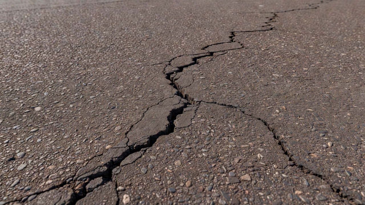
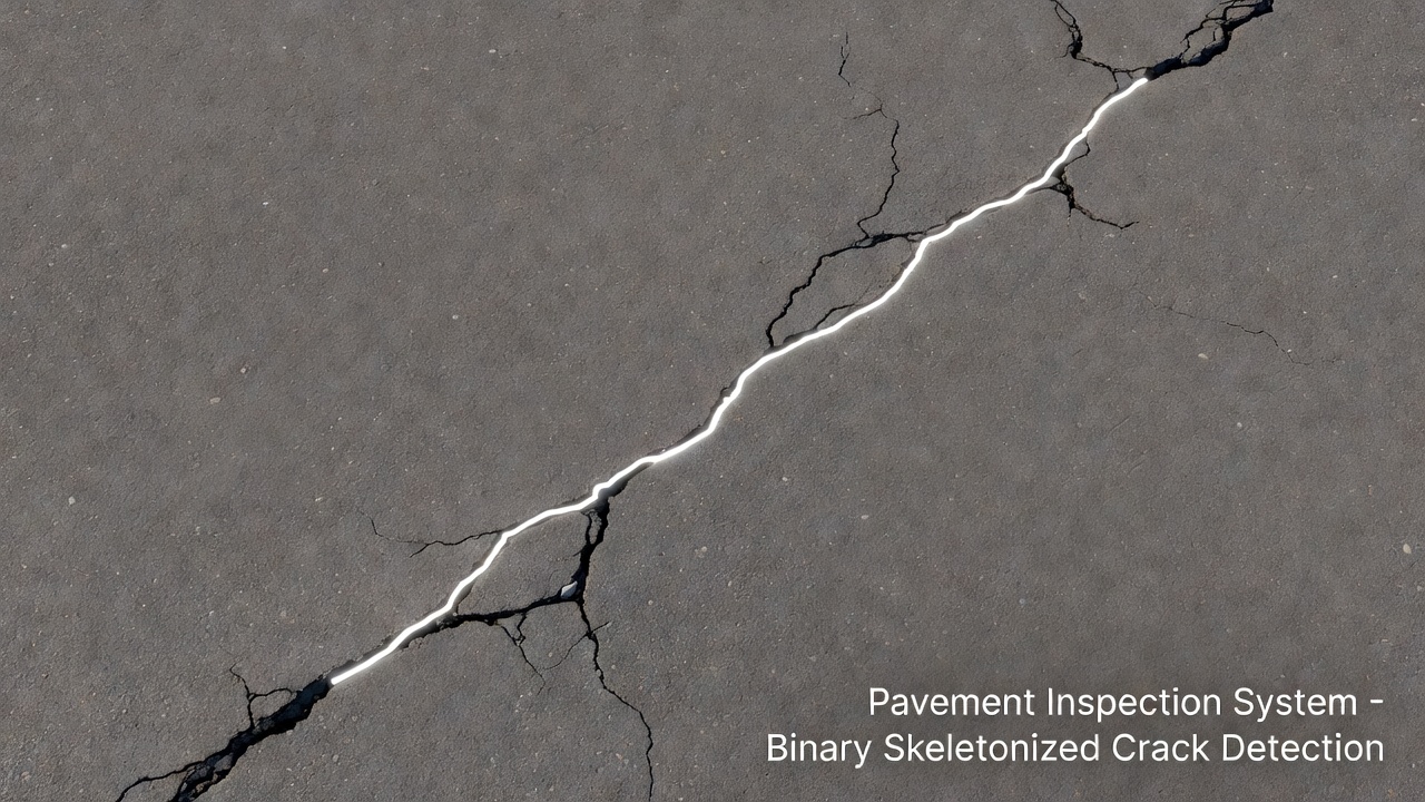
Crack skeletonization is the morphological image processing operation that reduces a segmented binary crack region to a single-pixel-wide centerline representation using thinning algorithms such as Zhang-Suen, Lee, or medial axis transform. The skeleton enables accurate crack length measurement, branching analysis, crack pattern classification, width estimation, and tortuosity quantification in automated pavement inspection systems.
Crack skeletonization (also referred to as thinning or medial axis extraction) is a morphological image processing operation that reduces a segmented binary crack region to a single-pixel-wide centerline representation — the skeleton — while preserving the topological properties (connectivity, branching structure) and geometric relationships (path shape, orientation) of the original crack. The skeleton represents the “centerline” or “medial axis” of the crack and is the foundation for virtually all quantitative crack geometry analysis in automated pavement inspection.
Formally, for a binary image I with crack pixels set to 1 (foreground) and background set to 0, skeletonization produces a set S ⊆ I with four essential properties. S is 1-pixel wide: every pixel in S has at most two 8-connected neighbors also in S, except at junctions where degree higher than 2 is allowed. S is topologically equivalent to I: S and I have the same number of connected components and the same hole/loop structure — the Euler characteristic is preserved. S is centered within I: each skeleton pixel lies approximately on the local midline of the crack. S is sufficient for reconstruction: in the case of the medial axis transform (MAT), the original shape can be approximately reconstructed from the skeleton plus its associated radius values.
In automated pavement crack analysis, skeletonization serves as a critical intermediate step between crack detection and segmentation and quantitative parameter estimation. The skeleton enables seven primary analytical functions. Crack length measurement is directly computed by tracing pixel paths along the 1-pixel-wide centerline. Crack width estimation uses the distance from skeleton pixels to crack boundaries to compute local and aggregate width statistics. Crack pattern classification detects junctions, branches, and topological structure to distinguish alligator, block, longitudinal, and transverse cracking. Crack orientation analysis determines the dominant crack direction per segment. Tortuosity quantification measures crack curvature and meandering as a ratio of skeleton path length to endpoint Euclidean distance. Data reduction compresses the crack region from hundreds or thousands of pixels to a compact linear representation that is computationally efficient for downstream analysis. Graph-based analysis converts the skeleton to a Euclidean graph with nodes representing junctions and endpoints and edges representing crack segments for advanced structural and topological analysis.
The skeleton provides a functional descriptor that bridges low-level pixel data and high-level engineering condition assessment parameters — crack length in meters, mean width in millimeters, crack density, and Pavement Condition Index (PCI) deductions as defined in ICAO ALACPA/09-2012, FAA PAVER, ASTM D5340-12, and ASTM D6433 standards.
Four primary algorithms are used for crack skeletonization: Zhang-Suen thinning, Guo-Hall thinning, Lee skeletonization, and the Medial Axis Transform (MAT). Each has distinct characteristics that make it suitable for different pavement analysis scenarios.
The Zhang-Suen (ZS) algorithm, published by T.Y. Zhang and C.Y. Suen in Communications of the ACM (Vol. 27, No. 3, March 1984), is the most widely used thinning algorithm in pavement crack analysis due to its speed, simplicity, and good results on elongated crack-like patterns. ZS is a parallel iterative thinning algorithm that operates on binary images by repeatedly removing border pixels while preserving connectivity.
The neighbor labeling convention for each pixel P1 under consideration arranges its eight neighbors in clockwise order: P9 (top-left), P2 (top-center), P3 (top-right), P8 (center-left), P4 (center-right), P7 (bottom-left), P6 (bottom-center), P5 (bottom-right). Two functions are defined for each black pixel P1: A(P1) equals the number of transitions from white (0) to black (1) in the ordered circular sequence P2 through P9 and back to P2, which measures the number of connected background components in the neighborhood; B(P1) equals the number of black pixel neighbors of P1.
ZS is a two-subiteration algorithm. Each iteration consists of two sequential steps. In Step 1, pixels on the north and east boundaries are marked for deletion; in Step 2, pixels on the south and west boundaries are marked. Only pixels that survive both sub-iteration conditions simultaneously are removed.
Step 1 conditions (mark for deletion): P1 is black foreground AND has 8 neighbors (not a border pixel of the image); 2 ≤ B(P1) ≤ 6 (ensures P1 is not an endpoint and not a thick interior pixel); A(P1) = 1 (preserves connectivity by preventing deletion of pixels that bridge multiple background components); P2 × P4 × P6 = 0 (at least one of east, south, or west neighbors is white); and P4 × P6 × P8 = 0 (at least one of north, east, or south neighbors is white). Conditions 4 and 5 together ensure that only north/east boundary pixels are removed in Step 1.
Step 2 conditions (mark for deletion): Conditions 1, 2, and 3 are identical to Step 1. Conditions 4 and 5 change to target south/west boundary pixels: P2 × P4 × P8 = 0 (at least one of north, east, or west neighbors is white) and P2 × P6 × P8 = 0 (at least one of north, south, or west neighbors is white).
The iteration process repeats until no pixels are deleted in either step. Deletions are made after each full pass to prevent removal order from affecting results (parallelism). The algorithm terminates when no pixels satisfy either Step 1 or Step 2 conditions. In practice, crack images typically require 5 to 15 iterations. The standard implementation uses a lookup table of 256 entries indexed by the 8-bit neighbor pattern for computational efficiency.
Zhang-Suen characteristics include preservation of 8-connectivity of foreground, very fast O(n) per iteration performance, production of skeletons that may retain some 2-pixel-wide diagonal lines, moderate noise sensitivity producing spurious branches (spurs) at boundaries of irregular crack regions (pruning is almost always required), and good but not perfect centering with slight bias toward certain boundary configurations.
The Guo-Hall (GH) algorithm, published by Z. Guo and R.W. Hall in Communications of the ACM (Vol. 32, No. 3, 1989), is another parallel two-subiteration thinning algorithm designed to address limitations of ZS — particularly the production of 2-pixel-wide diagonal lines and sensitivity to noise. GH uses two sub-iterations with the same structure as ZS but with different deletion conditions: odd iterations delete north-east boundary pixels (similar to ZS Step 1) and even iterations delete south-west boundary pixels (similar to ZS Step 2), using a more restrictive set of neighborhood conditions.
The Guo-Hall conditions for odd iteration require: P1 is black foreground; 2 ≤ B(P1) ≤ 6; A(P1) = 1; P2 × P4 × P6 = 0; and P4 × P6 × P8 = 0. For even iteration: P1 is black foreground; 2 ≤ B(P1) ≤ 6; A(P1) = 1; P2 × P4 × P8 = 0; and P2 × P6 × P8 = 0. GH adds a checking condition to prevent complete elimination of diagonal lines: the pixel is not deleted if it is the only remaining pixel connecting two otherwise disconnected skeleton components, determined by checking whether deletion would violate 8-connectivity using specific pattern matching.
| Property | Zhang-Suen | Guo-Hall |
|---|---|---|
| Skeleton thickness | May leave 2-pixel diagonal lines | Single-pixel throughout |
| Diagonal handling | Poor — produces thicker diagonals | Good — keeps 1-pixel diagonals |
| Runtime | Slightly faster | Comparable |
| Centering | Good | Good |
| Spur formation | Moderate | Slightly fewer spurs |
| Connectivity | Good | Better for thin features |
| Implementation | Simple | Moderate (additional checks) |
Per published benchmarks, GH produces thinner skeletons than ZS overall and better handles diagonal line patterns, but at marginally higher computational cost.
The Lee algorithm, published by T.-C. Lee, R.L. Kashyap, and C.-N. Chu in Computer Vision, Graphics, and Image Processing (Vol. 56, No. 6, 1994), extends thinning to 3-D binary images using an octree data structure to examine 3×3×3 neighborhoods. For 2-D crack analysis, it provides a useful alternative to ZS. When applied to 2-D images (as in scikit-image’s skeletonize(image, method='lee')), it follows the same fundamental principle of iterative border pixel removal but uses a two-phase approach per iteration: candidate identification (scanning all foreground border pixels and identifying those deletable based on template matching against a set of 256 3×3 patterns) and sequential rechecking (candidates are re-examined sequentially to verify that deletion does not break connectivity). This sequential rechecking is the key difference from ZS — it better preserves connectivity but is slightly slower.
Key properties of the Lee algorithm include superior preservation of connectivity compared to ZS for complex crack networks with multiple junctions, consistently 1-pixel-wide skeletons, slower speed for 2-D images due to the sequential rechecking phase (designed primarily for 3-D), and comparable or slightly better spur formation than ZS.
The Medial Axis Transform (MAT), introduced by H. Blum in Models for the Perception of Speech and Visual Form (MIT Press, 1967), is a fundamentally different approach from iterative thinning. It is based on the distance transform of the binary image. The medial axis of a binary object is the set of all points that have more than one closest point on the object’s boundary — equivalently, the locus of centers of maximal inscribed circles (disks) that fit entirely within the object.
Computation involves three steps. First, compute the distance transform: for each foreground (crack) pixel, calculate its Euclidean distance to the nearest background pixel, producing a distance map D(x,y). Second, identify ridge points: the medial axis consists of pixels that are local maxima in the distance transform — pixels whose distance-to-boundary value is greater than or at least equal to any of their neighbors. Third, threshold and thin: ridge points with distance values above a noise threshold form the initial skeleton, with additional thinning applied to ensure single-pixel width.
| Property | Iterative Thinning (ZS, GH, Lee) | Medial Axis Transform |
|---|---|---|
| Principle | Iterative border removal | Distance transform ridges |
| Centering | Good, approximate | Optimal — inherently centered |
| Width information | Requires separate computation | Built-in (distance values) |
| Computational cost | Fast (O(n) per iteration) | Moderate (distance transform) |
| Spur formation | Significant | Less spurious |
| Connectivity | Preserved | May produce disconnected components |
| Noise robustness | Moderate | Less robust to irregular boundaries |
| Skeleton smoothness | Can be jagged | Smoother overall |
For pavement crack analysis, thinning algorithms (especially ZS) are more commonly used because cracks are elongated, irregular structures where strict MAT centering is less critical and connectivity preservation is paramount.
Skeletonization inevitably produces spurious branches (also called spurs, hairs, or artifacts) — short side branches that do not correspond to real crack features but arise from noise, boundary irregularities, or aggregate texture in the pavement surface. The primary sources include boundary noise (small concave/convex perturbations in the crack boundary that get skeletonized as short branches), asphalt aggregate texture (grayscale variations near crack edges that cause the binary segmentation to have rough boundaries), salt-and-pepper noise (isolated misclassified pixels in the segmented image), and crack bifurcation artifacts (where varying crack width causes the skeleton to briefly split and rejoin).
The simplest and most widely used pruning technique is length-based pruning. The algorithm identifies all end-point pixels in the skeleton (pixels with exactly one 8-connected neighbor). For each end-point, it traces the branch back toward the main skeleton until a junction pixel (degree ≥ 3) is encountered. It then measures the branch length in pixels and removes the branch if its length is below a threshold T (typical threshold values range from 5 to 30 pixels depending on image resolution and crack characteristics). The process repeats until no further branches are pruned, since removing one branch may create new end-points. The length threshold is typically set based on pixel-to-mm calibration. For commonly used pavement imaging resolutions (0.5-2 mm/pixel), a threshold of 10-20 pixels corresponds to 5-40 mm, which effectively removes texture-induced noise while retaining real short crack branches.
Described in Li et al. (2023) for asphalt pavement crack analysis, the connected domain threshold method applies connected component labeling to the skeleton image, calculates the pixel count for each connected component, and removes components with pixel counts below a threshold (typically 50-200 pixels). This simultaneously removes isolated noise and short spurious branches from otherwise connected crack skeletons.
More sophisticated approaches consider additional criteria such as branch-to-skeleton angle (branches forming near-perpendicular angles to the main crack line are more likely to be spurious), branch thickness at origin (a branch emerging from a thick section of the skeleton is more likely to be real), distance transform value (branches whose distance transform values change abruptly are more likely to be noise), and contour continuity (if the branch has no corresponding indentation on the crack boundary contour, it is spurious).
Mathematical morphology offers direct pruning operators: MATLAB’s bwmorph(BW, 'spur', k) removes spur pixels with parameter k specifying iterations, and the hit-or-miss transform uses structural element matching to identify and remove specific spur patterns. The graph-based approach converts the skeleton to a graph with nodes (junctions and endpoints) and edges (pixel paths between nodes), assigns edge weights based on Euclidean distance, prunes edges whose weight is below a threshold and that connect to an endpoint (leaf edges), and additionally prunes short edges that connect two junctions if they create a small loop.
The Hybrid Skeleton-Prune-EOB method from a 2025 MDPI paper on concrete crack width measurement applies fast skeleton pruning using iterative endpoint tracing with length-based removal using an adaptive threshold based on mean crack width, followed by Edge-OrthoBoundary (EOB) reconstruction where the remaining skeleton undergoes boundary refinement to ensure accurate width measurement.
Accurate crack length measurement from the skeleton requires careful handling of pixel connectivity. The fundamental approach traces the skeleton path pixel by pixel and accumulates distances.
Starting from an endpoint (or junction-to-junction), the algorithm traverses along the 8-connected path. For each consecutive pair of pixels (x₁, y₁) and (x₂, y₂), the appropriate distance is added. Three distance metrics are available. 4-connected distance adds 1.0 for each orthogonal step (horizontal or vertical) but ignores diagonal connections, producing systematically longer lengths for diagonal crack segments. 8-connected (Chebyshev) distance adds 1.0 for each step in any of 8 directions, but this underestimates diagonal distance. Corrected 8-connected (Chamfer) distance adds 1.0 for orthogonal steps and √2 ≈ 1.414 for diagonal steps, yielding length measurements accurate to within approximately 0.5% of the true Euclidean path length.
The recommended approach for crack measurement uses 8-connected tracing with √2 correction:
def skeleton_length(skeleton_pixels):
    total_length = 0.0
    for i in range(len(skeleton_pixels) - 1):
        x1, y1 = skeleton_pixels[i]
        x2, y2 = skeleton_pixels[i+1]
        dx = abs(x2 - x1)
        dy = abs(y2 - y1)
        if dx == 1 and dy == 0 or dx == 0 and dy == 1:
            total_length += 1.0
        elif dx == 1 and dy == 1:
            total_length += sqrt(2)
    return total_length
For complex crack networks with branches, the skeleton is decomposed into segments between junction/endpoint nodes. All junction pixels (degree ≥ 3) and endpoint pixels (degree = 1) are detected. The skeleton is decomposed into segments between these nodes. Each segment is measured individually using the Chamfer distance method. Total crack length equals the sum of all segment lengths: L_total = Σᵢ Lᵢ where Lᵢ is the corrected 8-connected length of the i-th skeleton segment.
The practical implementation pipeline extracts the skeleton using Zhang-Suen thinning, prunes spurious branches (connected domain threshold, minimum 50-200 pixels), calibrates the pixel-to-mm ratio using a reference object of known dimensions imaged at the same distance, traces ordered skeleton pixels, applies Chamfer-distance accumulation, and converts to physical units: L_mm = L_pixels × scale_factor.
A junction pixel in a skeletonized crack image is a pixel with degree ≥ 3 — three or more neighboring skeleton pixels in an 8-connected neighborhood. For each skeleton pixel, the number of 8-connected neighbors is counted:
| Degree | Classification | Crack Interpretation |
|---|---|---|
| d = 0 | Isolated vertex | Noise (typically removed) |
| d = 1 | End vertex | Crack tip, branch end, or incomplete detection |
| d = 2 | Internal vertex | Continuation of a single crack segment |
| d = 3 | Branching vertex (T/Y) | Crack bifurcation |
| d = 4 | Branching vertex (X) | Crack intersection |
| d ≥ 3 | Junction vertex | General branching point |
In MATLAB, bwmorph(skel, 'branchpoints') detects pixels where the skeleton splits using a lookup table approach that examines the 3×3 neighborhood pattern against precomputed templates for branching configurations. This function may produce clusters of branch points around a single junction; these should be merged using connected component labeling and taking the centroid of each cluster.
From the graph representation, eight topological metrics can be computed. Number of junctions (J) per unit area — high J indicates a complex, interconnected crack network. Node degree distribution includes mean degree ⟨d⟩ = 2E/N (where E = number of edges, N = number of nodes), with a pure linear crack having ⟨d⟩ = 2 and a branching network having ⟨d⟩ > 2, and the degree ratio R_d = (degree-3+ nodes) / (degree-1 nodes). Number of branches (B) counts total skeleton segments between junction/endpoint nodes. Branch length statistics include mean branch length (shorter for alligator cracking, longer for longitudinal/transverse cracking), standard deviation (high for mixed cracking patterns), and coefficient of variation (used to distinguish block cracking from alligator cracking). Number of connected components (C) indicates either multiple distinct cracks or detection gaps. Euler number (χ) = C − H where H = number of holes (loops), with loops indicating alligator or block cracking. Fractal dimension (D_f) using the box-counting method on the skeleton yields approximately 1.0 for straight linear cracks, 1.2–1.4 for meandering cracks, and 1.5–1.8 for alligator cracking. Mesh size for block/alligator cracking — the average polygon area from cycle detection in the graph — indicates crack severity.
| Crack Pattern | Topological Signature |
|---|---|
| Longitudinal | Single main branch, few short side branches, d ≈ 2, low J |
| Transverse | Single main branch crossing the pavement, d ≈ 2, low J |
| Block | Polygonal network with ≥4-sided cycles, moderate J, medium-to-large mesh size |
| Alligator (Fatigue) | Dense network of small polygons, high J, high branch density, small mesh size, D_f ≥ 1.5 |
| Reflection | Linear cracks at regular intervals corresponding to underlying slab joints |
| Edge/Wheelpath | Localized cluster of cracks, often parallel to traffic direction |
For advanced topological characterization, Betti numbers provide further insight: β₀ equals the number of connected components (C), and β₁ equals the number of independent cycles or holes (H). The genus g = β₁ = H. Alligator cracking has high β₁, while simple linear cracks have β₁ = 0.

Crack width is a critical parameter for assessing pavement damage severity in standards such as ICAO ALACPA/09-2012, FAA PAVER, and ASTM D6433. The skeleton provides a natural reference for width measurement.
The most direct method uses the distance transform values at skeleton pixels. The Euclidean Distance Transform (EDT) of the binary crack image stores, for each foreground pixel, the Euclidean distance to the nearest background pixel. EDT values are extracted at all skeleton pixel positions. For each skeleton pixel, the local crack width = 2 × EDT_value (since EDT gives the radius to the nearest boundary). Statistics computed include mean width, max width, min width, and width standard deviation. Caveats include overestimation of width near skeleton endpoints (the EDT radius increases at crack tips where the distance extends around the tip curvature) and underestimation at junctions (the skeleton diverges from the true medial axis at branch points). Correction typically excludes the last 5-10 pixels at each endpoint.
A more accurate alternative accounts for local crack orientation. For each skeleton pixel (x₀, y₀), the local crack orientation θ is determined by fitting a line through neighboring skeleton pixels (typically ±3-5 pixels along the skeleton path). The normal direction is computed: θ_normal = θ + π/2. In the binary crack image, a profile along the normal from (x₀, y₀) outward in both directions is traced until background pixels are reached. The crack width equals the total distance (in pixels) between the two boundary intersection points along the normal. Implementation details include using bilinear interpolation for sub-pixel accuracy when profiling, setting profile length to exceed the expected maximum crack width (typically 50-100 pixels), and keeping the normal step size at ≤ 1 pixel for accurate boundary detection.
Advantages of perpendicular profiling include higher accuracy than the EDT method and better handling of non-circular crack cross-sections. Disadvantages include computational intensity and sensitivity to skeleton smoothness (jagged skeletons produce noisy orientation estimates).
Maximum crack width is a standard severity criterion in both ICAO and FAA pavement inspection manuals. To compute it, width is measured at every skeleton pixel (using EDT or profiling), and the maximum value is reported. Optionally, the width array is smoothed with a moving average (window of 5-11 pixels) to filter outliers before taking the maximum. Mean crack width averages width along the full skeleton excluding junctions and terminal segments for accuracy. Width distribution histogram characterizes crack uniformity and identifies locations of localized widening. Width coefficient of variation (CV = σ_w / μ_w): high CV indicates non-uniform cracking suggestive of spalling or edge deterioration.
Tortuosity (τ) quantifies the deviation of a crack from a straight line. It is defined as the ratio of the actual crack path length to the Euclidean (straight-line) distance between its endpoints:
τ = L_skeleton / L_euclidean
where L_skeleton is the total path length along the skeleton (using √2-corrected 8-connected distance) and L_euclidean is the Euclidean distance between the two endpoints of the crack segment.
Properties include τ ≥ 1.0 always (a straight line has τ = 1.0), τ = 1.0–1.05 indicating a nearly straight crack (typical of transverse or longitudinal thermal cracking), τ = 1.05–1.2 indicating a moderately meandering crack, τ = 1.2–1.5 indicating a highly tortuous crack (typical of alligator cracking secondary branches), and τ > 1.5 indicating an extremely tortuous path.
For crack networks with multiple branches, tortuosity is computed per crack segment (between consecutive junctions). For segment i with endpoints A(x₁,y₁) and B(x₂,y₂): τᵢ = L_skeletonᵢ / √[(x₂ - x₁)² + (y₂ - y₁)²]. Overall tortuosity for the crack network can be reported as mean segment tortuosity τ_mean = (1/N) Σᵢ τᵢ, maximum segment tortuosity τ_max = max(τᵢ), or global tortuosity using endpoints of the entire crack network (less meaningful for branched cracks).
Tortuosity is related to the fractal dimension (D_f) of the crack path. For a crack with fractal dimension D_f: τ ≈ K · (L_euclidean)^(D_f - 1) where K is a scaling constant. This relationship is used in fracture mechanics to relate crack tortuosity to material properties such as aggregate interlock and fracture energy. From Purdue research on crack tortuosity in concrete, tortuosity directly correlates with fluid permeability through the crack network — higher tortuosity leads to reduced effective flow area and lower permeability. For pavement applications, higher tortuosity cracks tend to retain less water and debris, affecting freeze-thaw damage potential.
Crack skeletonization operates as a post-processing step within a larger pavement crack analysis pipeline. The complete pipeline consists of six stages. Image acquisition captures pavement surface imagery using line-scan cameras, DSLR cameras, or mobile inspection vehicles at typical resolutions of 0.5-2 mm/pixel. Preprocessing applies normalization, contrast enhancement, and noise reduction to prepare the image for segmentation. Crack segmentation produces a binary mask of crack regions using deep learning models (U-Net, DeepLab, or Mask R-CNN) or traditional thresholding methods. Skeletonization reduces the binary mask to a single-pixel-wide centerline using Zhang-Suen, Guo-Hall, Lee, or MAT. Post-processing applies skeleton pruning to remove spurious branches, junction clustering to merge nearby branch points, and connected component analysis to separate distinct cracks. Parameter computation extracts length, width, tortuosity, branching metrics, and pattern classification from the cleaned skeleton.
The data flow processes the binary mask to skeleton to graph to parameters. Deep learning integration notes that modern systems use segmentation models trained on pixel-level crack annotations, with skeletonization applied to the model output. The quality of the skeleton depends heavily on the quality of the underlying segmentation — over-segmentation creates numerous spurious branches while under-segmentation produces disconnected skeletons. Joint training approaches that incorporate skeleton consistency losses (skeleton-aware segmentation) are an active research area.
Quantitative assessment of skeleton quality is essential for validating the performance of skeletonization algorithms in pavement crack analysis. Five primary metrics are used.
Completeness measures the proportion of the crack region that is represented by the skeleton. It is computed as the fraction of foreground pixels in the binary mask that are within a distance threshold (typically 2-5 pixels) of a skeleton pixel. A completeness value above 0.95 indicates the skeleton adequately captures the full extent of the crack.
Correctness (Precision) measures the proportion of skeleton pixels that lie within the actual crack region. It is computed as the fraction of skeleton pixels that are within the binary mask (considering a small tolerance for boundary effects). A correctness value above 0.98 indicates minimal hallucinated structure.
Skeleton IoU (Intersection over Union) combines completeness and correctness. It is computed by dilating the skeleton by a small radius (e.g., 2 pixels), computing the intersection with the binary mask, and dividing by the union. This provides a single scalar quality score typically ranging from 0.85 to 0.98 for well-performing algorithms.
Smoothness measures the curvature consistency of the skeleton path. It is computed using the mean rate of orientation change along the skeleton (angular deviation per pixel) or the number of inflection points per unit length. Lower values indicate smoother, more natural skeletons.
Connectivity verifies that the skeleton preserves the connectivity of the original crack. It is measured by counting the number of connected components in both the binary mask and the skeleton. The component count ratio (skeleton components / mask components) should be close to 1.0. The Euler characteristic error |χ_skeleton − χ_mask| measures topological consistency.
Centering error measures how well the skeleton represents the true medial axis. It is computed as the mean or RMS distance from skeleton pixels to the true medial axis (known for synthetic test cases) or to the contour midline (estimated for real images).
A composite quality assessment score can be computed as a weighted combination: Q = w₁Completeness + w₂Correctness + w₃(1 − NormalizedSmoothness) + w₄Connectivity, with weights adjusted for application requirements.
Several software libraries implement skeletonization algorithms suitable for crack analysis.
OpenCV provides cv2.ximgproc.thinning() in the extended image processing module. This function implements both Zhang-Suen (default) and Guo-Hall variants, selectable via the thinningType parameter. It operates directly on binary images and returns a single-pixel-wide skeleton. The function uses efficient lookup tables and is optimized for real-time applications.
scikit-image provides three skeletonization functions. skimage.morphology.skeletonize(image, method='zhang') implements Zhang-Suen thinning. skimage.morphology.skeletonize(image, method='lee') implements Lee’s algorithm with sequential rechecking. skimage.morphology.medial_axis(image, return_distance=True) computes the Medial Axis Transform and optionally returns the distance transform values for width estimation. All functions accept 2-D binary arrays and return binary skeletons.
MATLAB provides bwmorph(BW, 'skel', Inf) for skeletonization using the Zhang-Suen algorithm with infinite iterations, bwmorph(BW, 'branchpoints') for junction detection, bwmorph(BW, 'endpoints') for endpoint detection, and bwmorph(BW, 'spur', k) for iterative spur removal. MATLAB also provides bwdist() for the distance transform used in MAT-based approaches.
SciPy provides scipy.ndimage.distance_transform_edt() for computing the Euclidean distance transform, which is used with skeletonization for width estimation via the distance transform method.
| Tool | Function | Algorithm | Use Case |
|---|---|---|---|
| OpenCV | cv2.ximgproc.thinning() | ZS (default) or GH | Real-time crack analysis |
| scikit-image | skeletonize(method='zhang') | Zhang-Suen | General crack skeletonization |
| scikit-image | skeletonize(method='lee') | Lee | Complex crack networks |
| scikit-image | medial_axis() | MAT | Width-integrated analysis |
| MATLAB | bwmorph('skel', Inf) | ZS | Research and prototyping |
| MATLAB | bwmorph('branchpoints') | Junction detection | Pattern analysis |
| Fiji/ImageJ | Skeletonize3D plugin | ZS, Lee | 3-D crack analysis |
Fiji/ImageJ with the Skeletonize3D plugin (by Ignacio Arganda-Carreras) provides 2-D and 3-D skeletonization and is widely used in materials science for crack network analysis in X-ray CT imagery.
The International Civil Aviation Organization (ICAO) provides guidance on pavement crack inspection and measurement through several key documents. ICAO ALACPA/09-2012 (Airport Pavement Maintenance and Management) specifies crack measurement protocols including length measurement in meters using the centerline method (directly corresponding to skeleton-based measurement), width classification into severity levels (hairline: <3 mm, medium: 3-6 mm, severe: >6 mm), and pattern classification (longitudinal, transverse, block, alligator, reflection). ICAO Aerodrome Design Manual (Doc 9157, Part 3 — Pavements) references ASTM D5340-12 (Standard Test Method for Airport Pavement Condition Index Surveys) which requires crack density calculations (total crack length per unit area) and crack severity ratings based on width and pattern.
The FAA PAVER Distress Manual defines crack types with specific codes: longitudinal (L), transverse (T), block (B), alligator/fatigue (A), reflection (R), and edge (E). Severity thresholds are defined for width in inches: low severity (hairline to <1/4 inch), medium severity (1/4 to 1/2 inch), and high severity (>1/2 inch). Measurement protocols require recording crack length for linear cracks and square footage for area cracks. ICAO ALACPA and FAA PAVER require PCI computation using crack density (length per area), deduct values from standardized curves, and correction factors for multiple distress types. Skeletonization algorithms directly compute all required parameters: crack length (Section 4), mean width (Section 6), crack density (length per unit pavement area), and pattern classification (Section 5) for automated PCI deduction assignment.
For more information on implementing crack skeletonization in your pavement inspection workflow, contact our team or schedule a demo .
Leverage advanced crack skeletonization and geometry extraction for precise pavement condition assessment. Our computer vision solutions integrate skeleton-based length, width, and pattern analysis to deliver accurate PCI ratings and maintenance recommendations. Contact us for a demo of our automated inspection platform.
Automated crack width measurement derives the opening width of detected cracks from segmented pixel masks using Euclidean distance transform from crack edges to...
AI-based crack detection uses computer vision — convolutional neural networks, vision transformers, and semantic segmentation models — to automatically identify...
Crack segmentation is the computer vision task of classifying every pixel in an image as either crack or non-crack, producing a binary mask that enables precise...