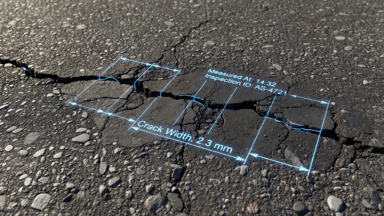
Automated Crack Width Measurement from Imagery

What is Automated Crack Width Measurement?

Automated crack width measurement is the computational process of deriving the opening width of detected cracks from digital imagery by converting segmented pixel masks into calibrated metric values. The measurement pipeline transforms raw pixel data through a series of algorithmic steps — binary segmentation to isolate crack pixels from the background, distance field computation or profile extraction to determine the separation between crack edges, and metric calibration to express the result in millimeters.

Crack width is the single most important quantitative indicator of crack severity in virtually every major pavement and concrete inspection standard. The width dimension directly correlates with structural degradation mechanisms — loss of load transfer across crack faces, ingress of water and chlorides, freeze-thaw damage potential, and progression toward spalling or raveling. While crack length indicates the extent of a defect, crack width determines its intensity and therefore its impact on structural performance and remaining service life.

The automated approach eliminates the subjectivity inherent in manual crack width measurement, where different inspectors may record different width values for the same crack depending on lighting conditions, comparator placement, and visual acuity. Algorithms produce deterministic, repeatable results — the same crack image processed through the same algorithm yields identical width measurements every time. This consistency is essential for longitudinal monitoring, where width changes over time indicate crack activity and the need for intervention.

Two principal algorithmic approaches dominate the field: the Euclidean Distance Transform (EDT) method, which computes width from the distance map of the segmented crack mask, and the Orthogonal Profile Extraction method, which samples intensity values along lines perpendicular to the crack centerline. Both approaches require metric calibration to convert pixel distances to millimeters and must account for edge irregularities, crack branches, and surface texture.

Importance for Severity Classification

Crack width classification directly drives maintenance decisions, repair prioritization, and budget allocation in infrastructure management. The severity of a crack determines not only whether repair is needed but also what type of repair is appropriate — narrow cracks may be sealed to prevent water ingress, while wide cracks may require structural filling or pavement replacement.

The structural implications of crack width are well-documented in the literature. Cracks wider than 0.3 mm (0.012 in.) in reinforced concrete allow chloride ions to reach the reinforcement and initiate corrosion, as defined by ACI 224R-01. Cracks exceeding 6 mm in asphalt pavements permit rapid water infiltration into the base and subgrade layers, accelerating structural deterioration through reduced support. Cracks wider than 19 mm create foreign object debris (FOD) hazards on airport runways and pose trip hazards for pedestrians, as noted in ICAO airport pavement evaluation standards.

The severity classification paradigm is hierarchical: crack width defines the severity band, while crack length or density at each severity level determines the extent of the defect. In the Pavement Condition Index (PCI) methodology per ASTM D6433-16, each distress type at each severity level has a corresponding deduct value that is subtracted from a perfect score of 100. A single wide crack may reduce the PCI by 5–15 points depending on density, while the same crack at low severity may reduce it by only 2–5 points.

AASHTO Crack Width Bands

The FHWA LTPP Distress Identification Manual (FHWA-HRT-13-092) is the authoritative reference for pavement crack severity classification in the United States. The manual defines three severity levels for asphalt concrete pavement cracks based on mean crack width, measured along the entire crack length.

These thresholds apply to block cracking, longitudinal cracking (both wheel-path and non-wheel-path), reflection cracking at joints, and transverse cracking in flexible pavements. The LTPP manual explicitly states that severity is based on mean width — a crack with intermittent wide sections but a low average width would be classified at lower severity than its widest point would suggest. This differs from bridge element inspection where maximum width governs.

For bridge deck inspections performed under AASHTO element-level inspection protocols, the crack width bands are significantly narrower, reflecting the more critical structural role of concrete bridge decks:

The bridge deck thresholds are 4–6 times stricter than pavement thresholds because bridge decks are structural elements directly subjected to live loads and environmental exposure. A 6 mm crack in a bridge deck would be classified as severe structural distress requiring immediate repair, whereas the same width in an asphalt pavement would be low-to-moderate severity.

For concrete structures under service loads, ACI Committee 224 has established allowable crack widths based on exposure conditions in ACI 224R-01. These are design limits rather than severity classifications, but they establish the thresholds above which structural concern is warranted:

The ICAO airport pavement classification defines low-severity cracks as predominantly 1 mm or less — hairline cracks and light shrinkage cracks. Airport runways are classified more strictly due to FOD concerns and the high cost of runway closures for repair.

Distance Transform Method for Width

The Euclidean Distance Transform (EDT) is the most widely used algorithmic approach for automated crack width measurement from binary segmented images. The transform converts a binary image — where foreground pixels represent the crack and background pixels represent the intact surface — into a grayscale distance map where each pixel’s intensity value equals the shortest Euclidean distance from that pixel to the nearest background pixel.

Mathematical Foundation

For a binary image I where I(p) = 0 for background and I(p) = 1 for foreground (crack pixels), the distance transform at pixel p is:

DT(p) = min{ d(p, q) | I(q) = 0 }

The Euclidean distance between pixels p with coordinates (x₁, y₁) and q with coordinates (x₂, y₂) is:

d(p, q) = √[(x₁ − x₂)² + (y₁ − y₂)²]

This produces a distance map where background pixels have DT value 0 and crack interior pixels have DT values proportional to their distance from the nearest edge. The maximum values within the crack region occur along the centerline, at the points farthest from both edges.

Processing Pipeline

The EDT-based crack width measurement follows a five-step pipeline:

Step 1 — Binary Segmentation: The crack is isolated from the background through thresholding, deep learning semantic segmentation (U-Net, DeepLab, or similar architectures), or manual annotation. The quality of this segmentation directly governs the accuracy of subsequent width measurements — errors in edge detection propagate linearly into width errors.

Step 2 — EDT Computation: For every pixel inside the crack region, the shortest Euclidean distance to the nearest non-crack pixel is computed. This can be performed in linear time O(N) using the Meijster/O’Rourke algorithm, a two-pass sequential raster scan that propagates distance values. The Felzenszwalb & Huttenlocher algorithm uses paraboloid intersection for exact Euclidean distances with the same linear complexity.

Step 3 — Skeleton Extraction: The crack centerline (medial axis or skeleton) is extracted, typically through morphological thinning (Zhang-Suen algorithm) or by identifying local maxima in the distance map. The skeleton represents the set of points equidistant (or maximally distant) from both crack edges. Each skeleton pixel is the point along the cross-section where the distance to both edges is equal.

Step 4 — Width Calculation: For each skeleton pixel, the crack width is calculated as:

Width(p_skel) = 2 × DT(p_skel)

The distance transform value at the skeleton gives the half-width — the shortest distance from the centerline to the nearest crack edge. Multiplying by 2 yields the full crack width at that cross-section.

Step 5 — Statistical Aggregation: The per-pixel widths along the skeleton are aggregated into summary statistics — mean, maximum, minimum, standard deviation, and coefficient of variation.

Algorithmic Implementation

The two-pass EDT for Manhattan (city-block) distance approximation:

Pass 1 — Top-left to bottom-right scan:

For each pixel (i, j):
    If I(i,j) == background: f[i][j] = 0
    Else: f[i][j] = INF
    If foreground: f[i][j] = 1 + min(f[i-1][j], f[i][j-1], f[i-1][j-1], f[i-1][j+1])

Pass 2 — Bottom-right to top-left scan:

For each pixel (i,j) in reverse order:
    f[i][j] = min(f[i][j], 1 + f[i+1][j], 1 + f[i][j+1],
                  1 + f[i+1][j-1], 1 + f[i+1][j+1])

The ImageJ implementation of this approach documents the relationship clearly: “The Distance Map shows for every pixel inside the crack the distance to its outer contour. The skeleton shows the maximum line. The product of Distance Map and Skeleton gives the half-width along the centerline.”

Orthogonal Profile Extraction

The Orthogonal Profile Extraction method approaches crack width measurement from a fundamentally different angle — rather than computing a distance field across the entire crack mask, it extracts one-dimensional intensity profiles along lines perpendicular to the crack centerline and determines the edge positions within each profile.

Why Orthogonality Matters

Crack width must be measured perpendicular to the crack centerline at each measurement point. Any measurement taken at a non-orthogonal angle overestimates the true width by a factor of 1/cos(θ), where θ is the deviation angle from the perpendicular. A 30-degree deviation produces a 15% width overestimate; a 45-degree deviation produces a 41% overestimate. This geometric error compounds along curved crack paths where the crack direction changes continuously.

Implementation Sequence

Step 1 — Skeleton Extraction: The crack centerline is obtained through medial axis transform or morphological skeletonization. For complex crack networks with branches and junctions, connected component analysis may separate individual crack segments before skeleton extraction.

Step 2 — Tangent Direction Computation: At each skeleton point, the local tangent (direction of crack propagation) is computed. Common methods include the derivative of a spline fitted to skeleton points, the direction of the eigenvector of the Hessian matrix of the distance map, or finite difference using neighboring skeleton points:

θ(s) = atan2(dy/ds, dx/ds)

Step 3 — Normal Direction Computation: The orthogonal profile direction is perpendicular to the tangent:

n_x = -sin(θ) n_y = cos(θ)

Step 4 — Profile Sampling: Pixel intensity values are sampled along the normal direction on both sides of the skeleton point. For subpixel accuracy, bilinear or bicubic interpolation is used to estimate intensity values at non-integer positions along the profile.

Step 5 — Edge Detection: The crack edges are located within each profile using threshold crossing, gradient peak detection, or subpixel interpolation techniques. The distance between the two detected edges is the crack width at that location.

Advanced Methods

The OrthoBoundary (EOB) algorithm, described in recent literature (Li et al., 2025), leverages both crack boundary direction and skeleton direction to eliminate systematic errors that occur at crack intersections and junctions. Traditional orthogonal profile methods produce erroneous width values at Y-junctions and X-junctions where a single skeleton point corresponds to multiple crack boundaries. The EOB method resolves these ambiguities by considering the boundary contour direction in addition to the skeleton direction.

The Neighborhood Shortest Distance (NSD) method (Liu et al., 2025) addresses the incorrect orthogonal projection problem at crack boundary intersections by considering the local neighborhood around each measurement point. Rather than treating each profile independently, the NSD method accounts for the variation in crack boundary direction across the local neighborhood, producing robust width measurements even where boundaries are irregular or where cracks branch.

Pixel-to-Metric Calibration

The conversion from pixel measurements to physical millimeters is the critical enabling step that transforms image-based analysis into actionable engineering data. Without accurate calibration, a 20-pixel-wide crack on a close-up image may represent either a 0.5 mm hairline crack or a 10 mm wide structural crack, depending on the imaging geometry.

Calibration Methods

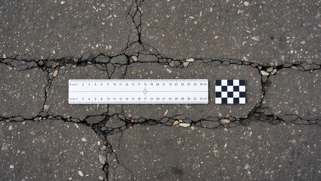
Method A — Reference Object / Scale Target: A calibration object of known physical dimensions is placed on the surface at the same distance from the camera as the crack. The object is detected in the image, and its pixel dimension is measured. The calibration factor is:

Calibration Factor (mm/pixel) = Known Physical Dimension (mm) / Measured Pixel Dimension (pixels)

Common reference objects include coins (standardized diameters), coded survey targets, checkerboard patterns, and scale bars with graduation marks. For concrete crack measurement, studies (Guo et al., 2023) report average errors of 0.26–0.71 mm for cracks under 5 mm using this method with proper lighting and target placement.

Method B — Camera Geometry (Pinhole Model): When the camera parameters are known and the distance to the surface can be measured, the calibration factor is derived from:

mm/pixel = (Sensor Width in mm × Working Distance in mm) / (Focal Length in mm × Image Width in pixels)

This method requires the focal length (from lens specification or camera calibration), sensor dimensions (from manufacturer specifications), and the distance from the camera to the surface (measured or estimated). It works well for controlled setups like gantry-mounted cameras or drones at known altitudes.

Method C — 3D Photogrammetry: For complex structures where the distance from camera to surface varies across the image (bridges, curved pavements, retaining walls), 3D point cloud reconstruction from stereo imagery or structure-from-motion (SfM) provides spatially varying pixel scales. The image is gridded into sections, and each section receives its own calibration factor based on the local 3D geometry.

Method D — Known Dimension in Scene: If the crack image contains any object of known physical size (e.g., manhole cover, pavement marking width, joint gap, utility cover), that object can serve as a reference. This method is less precise than Method A but enables retroactive calibration when no reference target was placed during image capture.

Critical Considerations

Resolution requirements: For measuring cracks below 0.3 mm (the ACI durability threshold), the pixel resolution must be better than 0.1 mm/pixel. At 0.1 mm/pixel, a 0.3 mm crack spans only 3 pixels, limiting the precision of the measurement. Subpixel techniques can partially overcome this limitation but cannot compensate for fundamentally inadequate resolution.

Orthogonality: The camera optical axis should be perpendicular to the surface within ±5 degrees to avoid perspective distortion. Larger angles require perspective correction through homography transformation, adding complexity and potential error sources.

Depth variation: On curved surfaces (pavement crowns, bridge girders, tunnel linings), the pixel scale varies across the image. A single calibration factor applied to the entire image introduces systematic errors proportional to the depth variation. Laser profiling systems (e.g., LCMS-2, Pavemetrics) solve this by using line laser illumination with known geometry, achieving 1 mm spatial resolution at highway speeds (up to 100 km/h).

Mean vs Maximum Crack Width

The choice between reporting mean crack width and maximum crack width has significant implications for severity classification and repair decision-making. Different standards mandate different statistical measures, and the two metrics can produce divergent severity ratings for the same crack.

Definitions

Per-skeleton-point width W(p) — The crack width calculated at each individual pixel along the skeleton centerline, whether through the EDT method (W(p) = 2 × DT(p)) or orthogonal profile extraction.

Maximum crack width W_max — The single largest width value along the entire crack:

W_max = max{ W(p) | p ∈ skeleton }

Mean crack width W_mean — The arithmetic average of all width measurements along the skeleton:

W_mean = (1/N) × Σ W(p_i) for all skeleton pixels i = 1…N

Usage in Standards

The FHWA LTPP Distress Identification Manual explicitly defines severity thresholds based on mean crack width. A crack with a local maximum width of 24 mm but a mean width of 5.5 mm would be rated LOW severity under LTPP rules because the average falls below the 6 mm threshold. The rationale is that the overall structural condition relates more closely to average degradation than to isolated wide spots.

Bridge element inspection protocols under AASHTO and the Pavemetrics Simplified AASHTO system use maximum crack width for severity classification. This approach is more conservative — a single wide section governs the severity of the entire crack. The rationale for this approach is that the widest point represents the worst-case condition for structural assessment, load transfer degradation, and water infiltration.

Statistical Behavior

The relationship between mean and maximum width depends on the width uniformity of the crack:

• For uniform-width cracks (constant opening along the crack path): W_mean ≈ W_max
• For tapered cracks (narrowing or widening along the path): W_max = 2–3 × W_mean
• For highly irregular cracks (localized wide spots): W_max may reach 5 × W_mean
• The coefficient of variation (CV = σ/μ) of the width profile characterizes crack irregularity — a CV > 0.3 indicates significant width variation that should be noted in the inspection report.

Width Measurement Accuracy and Uncertainty

The accuracy of automated crack width measurement is governed by a hierarchy of factors spanning image acquisition, segmentation quality, and algorithmic precision. Understanding these error sources is essential for interpreting width data and making informed decisions.

Achievable Accuracy Benchmarks

Subpixel Accuracy Techniques

Partial Area Effect (PAE): The PAE method models the area fraction of foreground within each boundary pixel to locate crack edges at subpixel resolution. A boundary pixel that is 60% crack and 40% background has its edge position estimated at 0.6 pixels from the boundary. This technique achieves measured accuracy of 0.01 pixels for crack length and absolute errors below 0.30 mm for crack width. The method works effectively for vertical, horizontal, and oblique crack orientations.

Least-Squares Matching (LSM): LSM applies an 8-parameter affine transformation for subpixel displacement estimation in image sequences, enabling crack propagation measurement over time. It achieves displacement precision of 0.1–0.2 pixels, with median errors of 0.021 pixels when model extensions are applied (compared to 0.088 pixels without).

Zernike Moment Method: This approach uses Zernike orthogonal moments for subpixel edge detection, particularly effective for thin cracks in images with complex backgrounds or varying illumination.

Factors Affecting Precision

Uncertainty Quantification Framework

The FHWA vendor selection guidelines (FHWA-RC-20-0005) establish a statistical framework for validating crack measurement systems. The protocol uses:

• Paired t-test for equivalence comparing vendor measurements against ground reference measurements
• Acceptance limits of ±4% to ±7.5% for HPMS cracking percentage
• Power analysis with assumed standard deviation of 5–10%
• Minimum 10 subsections per test section for statistical validity

For bridge inspections, ACI Committee 224 recommends reporting width measurements with confidence intervals, particularly for cracks near the severity thresholds where classification decisions hinge on measurement precision.

Crack Width in Structural Defect Assessment

Crack width is not merely a classification metric — it is a direct indicator of structural degradation mechanisms and potential failure modes. The relationship between width and structural performance is governed by physical mechanisms that vary across material types and structural configurations.

Degradation Mechanisms by Width Threshold

Research Findings on Width vs. Performance

Research from the University of Texas at Austin (CTR 0-6919-1) demonstrated that diagonal crack widths alone do not serve as reliable indicators of shear distress in concrete bridge girders. Mechanical properties and load testing are necessary for shear capacity assessment. However, flexural crack widths do correlate with steel stress and can be predicted using AASHTO equations (Gergely-Lutz and Kaar-Mattock formulations), providing a non-destructive method for estimating stress levels in the reinforcement.

An important consideration for repair decisions is that surface crack width does not equal internal crack width. Concrete cracks typically have V-shaped profiles — wider at the surface and narrower in the interior. This means surface measurements overestimate internal width, potentially leading to overly conservative repair decisions if not properly accounted for.

The ACI Committee 224 consensus guideline for structural assessment establishes these thresholds:

• Cracks below 0.1 mm (0.004 in.): Generally cosmetic, no structural concern
• Cracks 0.1–0.3 mm (0.004–0.012 in.): Monitor; may affect durability in aggressive environments
• Cracks 0.3–0.5 mm (0.012–0.020 in.): Requires evaluation; likely repair needed in severe exposures
• Cracks above 0.5 mm (0.020 in.): Generally requires repair; structural assessment needed

For epoxy injection repair, bond strength tests show that epoxy achieves bond strength exceeding concrete tensile strength for cracks as narrow as 0.05 mm (0.002 in.) — meaning even hairline cracks can be effectively repaired through injection methods.

Reporting Crack Width

Consistent, standardized reporting of crack width measurements is essential for condition assessment databases, longitudinal monitoring programs, and cross-agency data comparison. Different standards prescribe different reporting protocols.

Standard Reporting Protocols

FHWA LTPP / AASHTO PP67-10 Protocol:

• Report mean width for severity classification
• Record severity level (low/moderate/high) for each crack segment
• If severity varies along a crack, record each segment separately
• For transverse cracks: rate the entire crack at the highest severity present for 10% or more of the total crack length
• Report crack length in meters at each severity level

Bridge Element Inspection (AASHTO):

• Report maximum width for element condition state assignment
• Classify as Narrow (<1.6mm), Moderate (1.6–3.2mm), or Wide (>3.2mm)
• Report quantity of affected area at each condition state
• Record associated defects (spalling, efflorescence, exposed reinforcement)

ASTM D6433-16 (PCI) Protocol:

• Record crack density (length or area affected) at each severity level
• Apply deduct values based on density × severity
• Calculate PCI = 100 − total deduct value
• Report final PCI score and associated condition rating

ACI 224.1R-07 (Concrete Structures) Protocol:

• Report crack width to 0.025 mm (0.001 in.) precision when using microscope
• Document: location, length, width orientation, pattern
• Note crack activity: active (changing width over time) vs. dormant (stable)
• Record environmental exposure conditions
• Include photographic documentation

Essential Report Elements

A comprehensive crack width report should include:

1. Crack identification — Unique ID, structure element, station/offset coordinates
2. Width measurement — Reported width value (specify mean or maximum)
3. Measurement method — Comparator, microscope, automated EDT, orthogonal profile
4. Severity classification — Per governing standard (AASHTO, ASTM, ACI, ICAO)
5. Spatial extent — Length or area affected at each severity level
6. Crack orientation — Longitudinal, transverse, diagonal, map, alligator, block
7. Associated distress — Spalling, raveling, pumping, efflorescence, rust staining
8. Environmental class — Exposure conditions (dry, moist, deicing, marine)
9. Calibration data — mm/pixel factor, reference object details, camera parameters
10. Date and inspector — Inspection date, personnel, equipment used

Comparison with Manual Crack Comparator Measurement

Understanding the differences between automated and manual crack width measurement is essential for transitioning inspection programs from traditional to digital workflows. Both approaches have strengths and limitations that affect data quality, consistency, and cost.

Manual Measurement Methods

Crack Comparator Cards: Transparent, credit card-sized plastic cards printed with graded lines from 0.1 mm to 7.0 mm (0.004–0.26 in.). The Gilson HM-639 comparator covers the full range for approximately $4 per card. The user places the card over the crack and visually matches the printed line width to the crack opening. Typical accuracy is approximately ±0.5 mm, heavily dependent on lighting conditions, operator eyesight, and crack edge definition. The method is subjective — two inspectors may select different matching lines for the same crack.

Crack Width Rulers: The Elcometer 143 offers a range of 0.10–2.50 mm (0.004–0.100 in.) in a credit card-sized format. Line widths are specified and labeled, enabling direct visual comparison. Similar to comparator cards, accuracy depends on the inspector’s visual acuity.

Pocket Microscope with Reticle: Hand-held lighted magnifying microscope with an internal measurement scale offering precision to 0.025 mm (0.001 in.) per ACI 224.1R-07. This is the most accurate manual method, recommended by ACI Committee 224 for critical measurements. The microscope requires operator training, a stable surface, and adequate lighting — factors that limit its practicality for high-throughput field inspections.

Feeler Gauges: ACI Committee 224 explicitly discourages the use of feeler gauges for concrete crack measurement. The committee notes: “Crack widths and surfaces tend to be so irregular that a flat object would get hung up on irregularities and would underestimate measured crack widths.” Surface cracks typically exhibit notched profiles and raveled edges, meaning a feeler gauge measures the notch width at the surface rather than the true crack width below the surface.

Crack Monitors (Ongoing Measurement): Two overlapping plastic tabs mounted across a crack, with measurement grids enabling tracking of width changes over time. Resolution can reach 0.003 mm (0.00012 in.) with electronic data loggers. These devices distinguish active cracks (changing width) from dormant cracks (stable width), which is critical for prioritizing repairs.

Automated vs. Manual — Quantitative Comparison

Validation Results

A validation study comparing manual and digital measurement at Virginia Tech reported:

The photogrammetry combined with CNN approach (Guo et al., 2023) reported average errors of 0.26–0.71 mm for cracks under 5 mm when comparing automated measurements against manual ground truth.

The Elcometer 143 datasheet demonstrates that even the finest comparator cards are limited to 0.10 mm resolution at their finest lines. In contrast, subpixel image methods can detect width changes of 0.001–0.005 mm — two orders of magnitude more sensitive — making automated methods superior for detecting subtle width changes in crack monitoring applications.

ACI Committee 224 Position

The ACI Committee 224 FAQ on crack measurement provides definitive guidance:

“The only accurate measurement is through the use of a lighted magnifying microscope… For the novice and for field observation, the plastic graduated transparent pocket card is typically appropriate… Remember, we are talking about measuring crack widths in the range of 0.005 to 0.05 in. (0.127 to 1.27 mm).”

On feeler gauges:

“A feeler gauge will not give the user information about the width of the actual crack, but only the width of the notch at the surface.”

The committee recommends optical microscope with dedicated light source for accuracy-critical measurements, a recommendation that aligns with the trend toward digital imaging with controlled illumination in automated systems. The convergence of high-resolution cameras, powerful algorithms, and standardized lighting makes automated crack width measurement the preferred method for modern inspection programs requiring consistent, defensible, and permanent data.