Transfer Learning
Transfer learning applies knowledge from a model pre-trained on large general datasets (ImageNet 1.2M images, DINOv3 on 1.7B images) to specialized infrastructu...
23 min read
Technology
Machine Learning
+2
Data augmentation synthetically expands training datasets by applying image transformations — rotation, flipping, color jitter, blur, noise, cropping — to improve model robustness to variations in lighting, orientation, and image quality. For infrastructure inspection, domain-specific augmentations (perspective transforms, shadow simulation, weather effects) are critical. Covers augmentation strategies and their impact on model generalization.
{
Data augmentation is a training methodology that synthetically expands the size and diversity of a labeled dataset by applying controlled, label-preserving transformations to existing data samples. In computer vision applications, this means taking each original image and generating multiple modified versions through geometric warping, color-space manipulation, noise injection, or more complex generative processes. The augmented dataset — original images plus their transformed variants — is then used to train deep neural networks, exposing the model to a far wider range of visual conditions than the raw field data alone would provide.
The core purpose of data augmentation is to improve model generalization — the ability of a trained model to perform accurately on data it has never seen before. A deep convolutional neural network (CNN) with millions of parameters can easily memorize a training dataset of a few thousand images, learning the specific textures, lighting patterns, and background artifacts of those examples rather than the underlying defect signatures. This phenomenon, known as overfitting, results in high training accuracy but poor validation and test performance. Data augmentation prevents overfitting by ensuring that every training epoch presents the model with differently transformed versions of each image, making pure memorization impossible. The model is forced to learn invariant features — visual patterns that persist across transformations.
For infrastructure inspection models, data augmentation is not merely beneficial but operationally essential. Consider the data collection realities of airfield pavement inspection: a single runway survey using a UAV-mounted camera might capture 10,000 high-resolution images, but fewer than 200 of those images may contain visible defects. Cracks, spalls, joint sealant failures, and surface weathering together constitute less than 1 percent of the total pavement surface area at any given time. Collecting a balanced, diverse dataset of defects under all possible inspection conditions — direct sunlight, overcast, dawn, wet pavement, dry pavement, different camera pitch angles, different altitudes — would be prohibitively expensive and time-consuming. Data augmentation bridges this gap by simulating the full envelope of operational conditions from a much smaller set of field-collected examples.
The importance of augmentation is formally recognized across aviation infrastructure standards. ICAO Annex 14, Volume I (Aerodrome Design and Operations) requires that runway surfaces be maintained in a condition that does not endanger aircraft operations. AI-based inspection systems interpreted under these standards must demonstrate robust performance across the full range of operational lighting and weather conditions specified in the aerodrome manual. Without comprehensive augmentation, an inspection model trained exclusively on dry, midday captures would fail to detect cracks obscured by shadows, wet patches, or low-angle sunlight — potentially missing defects that compromise aircraft braking performance and operational safety.
Data augmentation operates at the data level rather than the model architecture level, distinguishing it from regularization techniques like dropout, weight decay, or batch normalization. While model-level regularizers constrain the network’s capacity to overfit, augmentation expands the data distribution to more completely cover the real-world input space. The two approaches are complementary: best practice infrastructure inspection pipelines combine aggressive augmentation with architectural regularization for maximum generalization.
Geometric augmentations modify the spatial arrangement of pixels in an image without altering their intensity values. These transforms simulate changes in camera position, orientation, distance, and lens characteristics that occur during real inspection data collection. For infrastructure inspection, geometric augmentations are the most impactful category because inspection platforms — UAVs, ground vehicles, handheld cameras — capture the same surface from widely varying perspectives.
Rotation augmentation applies a random angular rotation to the input image, typically ranging from -180° to +180° or constrained to smaller ranges such as ±45° for specific applications. The transformed image is generated by rotating every pixel coordinate (x, y) by angle θ about the image center using the standard rotation matrix:
x’ = x·cos(θ) - y·sin(θ)
y’ = x·sin(θ) + y·cos(θ)
For crack detection on airport runways and highway pavements, rotation augmentation is critical because the orientation of cracks relative to the camera frame is arbitrary. A longitudinal crack parallel to the runway centerline may appear horizontal in one image tile and diagonal in another, depending on the camera’s yaw angle relative to the aircraft landing direction. Without rotation augmentation, a model may learn to associate crack presence with a particular angular orientation, failing to detect cracks that appear at other angles. Research by Alomar et al. (2023) demonstrates that rotation augmentation consistently improves classification accuracy by 3-8 percent on structural defect datasets compared to models trained without rotation.
The optimal rotation range depends on the application symmetry. For airfield pavements where cracks develop in both longitudinal and transverse directions relative to aircraft traffic, a full ±180° range is appropriate. For bridge girder inspections where the camera is always roughly horizontal, a tighter ±15° range may be sufficient. Rotation introduces empty border regions at the image corners, which must be handled through one of three strategies: (1) zero-padding (filling borders with black), (2) reflection padding (mirroring edge pixels), or (3) nearest-neighbor padding. Reflection padding is preferred for infrastructure inspection because it avoids introducing artificial dark borders that the model could learn as spurious features.
Horizontal flip (mirroring left-right) and vertical flip (mirroring top-bottom) are the simplest geometric augmentations, requiring only a reversal of pixel column or row order. Horizontal flip is applied with 50 percent probability as a default in most augmentation pipelines and is universally beneficial because it doubles the effective dataset size while being computationally free — it requires no interpolation.
For infrastructure inspection, horizontal flipping preserves the label for most defect types. A crack is a crack regardless of whether it appears on the left or right side of the image. However, some defects have directional asymmetry: raveling (loss of aggregate at pavement edges) tends to occur preferentially along the pavement edge, and faulting (vertical displacement across a joint) has a directionality related to traffic loading. For these directional defects, the practitioner must verify that the flipped version remains a valid training example.
Vertical flipping is less commonly used for terrestrial infrastructure inspection because it inverts the gravity-consistent orientation of the image. A crack on a vertical concrete wall appears fundamentally different when flipped — though for pavement inspection where the camera is looking straight down, vertical flip is as label-preserving as horizontal flip. For bridge inspection imagery where the camera captures vertical surfaces (girders, piers, abutments), horizontal flip should be prioritized over vertical flip.
Random cropping selects a rectangular sub-region of the input image and resizes it to the network’s expected input dimensions. This simulates the effect of the camera being positioned at different distances from the surface being inspected — closer crops correspond to higher-resolution views with more detail, while wider crops show broader context.
The standard random-crop augmentation samples a crop region with an area between min_scale and max_scale (typically 0.08 to 1.0 of the original image area) and an aspect ratio between min_ratio and max_ratio (typically 0.75 to 1.33). The cropped region is then resized to the fixed network input size, for example 512×512 pixels for typical crack segmentation models.
For infrastructure inspection, random cropping serves a dual purpose. First, it increases positional diversity — a model trained only on full-frame images may learn to associate defects with their position within the frame, failing when the same defect appears in a different frame region. Second, cropping with resizing simulates different inspection altitudes and zoom levels, which is critical for UAV-based inspection where flight altitude varies between 10 meters and 50 meters depending on regulations and survey requirements. ICAO Doc 9137, Part 9 (Airport Maintenance Practices) and ICAO Doc 9981 (PANS-Aerodromes) address inspection methods that may involve vehicle-mounted or handheld data collection, each introducing different fields of view. Random cropping during training ensures the model generalizes across these capture modalities.
Perspective transformations (also called perspective warps or homography augmentations) apply a projective mapping to the image, simulating the effect of the camera plane being tilted relative to the surface being inspected. This is mathematically represented by a 3×3 homography matrix that maps points from one plane to another.
For infrastructure inspection, perspective augmentation is uniquely important because real inspection imagery is rarely captured from a perfectly orthogonal (nadir) viewpoint. Vehicle-mounted cameras capture pavement at a slight forward angle. UAV cameras may have pitch angles of 5-20 degrees as the drone maneuvers. Handheld inspection cameras vary in tilt depending on the inspector’s height and arm position. A crack that appears linear and consistent from a nadir view becomes foreshortened and geometrically distorted from an oblique angle. Perspective augmentation trains the model to recognize defects regardless of the capture angle.
The degree of perspective distortion is controlled by the distortion scale parameter, typically set between 0.05 and 0.3 in normalized coordinates. Higher values simulate more extreme camera tilts. For airfield inspection, a perspective scale of 0.1-0.2 is recommended, corresponding to camera pitch angles of approximately 5-15 degrees from nadir.
Affine transformations combine scaling, shearing, rotation, and translation into a single 2×3 matrix operation. Unlike perspective transforms, affine transforms preserve parallelism — parallel lines remain parallel after transformation. The operation can be expressed as:
[x’, y’]² = A · [x, y]² + b
where A is a 2×2 matrix controlling rotation, scaling, and shear, and b is a translation vector.
For infrastructure inspection, a common affine augmentation configuration includes: translation (±10 percent of image dimensions, simulating frame misalignment), scaling (0.8x to 1.2x, simulating altitude variation), shearing (±10 degrees, simulating camera tilt), and rotation (±15 degrees). The combined effect produces images that realistically simulate the positional and orientation variability of inspection data collection without requiring extreme distortions that might introduce unrealistic artifacts.
| Augmentation Type | Typical Range | Application for Infrastructure |
|---|---|---|
| Rotation | ±45° to ±180° | Simulates different camera yaw angles relative to crack orientation |
| Horizontal Flip | 50% probability | Doubles dataset; invariant for most defects |
| Vertical Flip | 50% probability | Useful for nadir pavement imagery |
| Random Crop | 0.08-1.0 scale, 0.75-1.33 aspect | Simulates different inspection altitudes and zoom levels |
| Perspective | 0.05-0.3 distortion scale | Simulates non-nadir camera tilt angles |
| Affine (scale) | 0.8x-1.2x | Simulates altitude variation of UAV platforms |
| Affine (shear) | ±5° to ±15° | Simulates camera roll and pitch |
| Affine (translate) | ±5% to ±15% | Simulates frame position variation |
| Affine (rotation) | ±10° to ±30° | Combined with other affine parameters |
{
Color and photometric augmentations modify the pixel intensity values of an image without changing the spatial arrangement of objects. These transforms simulate variations in lighting conditions — the most significant source of real-world variability in infrastructure inspection imagery.
Brightness augmentation linearly shifts all pixel values by adding a constant offset: I’ = I + δ, where δ is sampled uniformly from a range such as [-30, +30] on a 0-255 scale. This simulates the difference between midday sunlight (high brightness) and overcast sky or early morning inspection conditions (low brightness). Contrast augmentation scales pixel values around the mean intensity: I’ = α(I - μ) + μ, where α is sampled from a range such as [0.7, 1.3]. Lower contrast values simulate hazy or foggy conditions; higher values simulate harsh direct sunlight that produces strong shadows.
For infrastructure inspection, the recommended brightness range is ±40 percent to cover the full spectrum of operational lighting conditions specified in aerodrome lighting plans per ICAO Annex 14, Chapter 5 (Visual Aids for Navigation). Runway edge lighting, approach lighting, and apron flood lighting all create different ambient illumination levels that the inspection model must handle.
Hue shift rotates all pixel colors in HSV (Hue, Saturation, Value) color space by a random angle, typically ±30° out of a 360° color wheel. Saturation adjustment multiplies the saturation channel by a random factor (typically 0.5 to 1.5). These augmentations simulate the effect of different pavement surface conditions — dry asphalt has lower saturation than wet asphalt, aged concrete differs in hue from new concrete, and rubber tire deposits create distinct color artifacts on runway touchdown zones.
For crack detection on asphalt pavements, hue augmentation is particularly helpful because the contrast between a dark crack and the surrounding pavement varies with surface moisture. A dry hairline crack may have minimal color contrast against dry asphalt, while the same crack filled with water after rain appears as a clearly defined dark line. Models trained with hue and saturation augmentation learn to detect cracks across this moisture-driven contrast range.
Color jitter is a composite augmentation that randomly adjusts brightness, contrast, saturation, and hue simultaneously. The standard implementation samples each parameter independently: brightness factor in [1-δ_b, 1+δ_b], contrast factor in [1-δ_c, 1+δ_c], saturation factor in [1-δ_s, 1+δ_s], and hue rotation in [-δ_h, +δ_h]. For infrastructure inspection, the recommended ranges are δ_b=0.3, δ_c=0.3, δ_s=0.2, and δ_h=0.1.
Color jitter is a highly effective regularizer for defect detection models. Research on pavement crack classification shows that models trained with comprehensive color jitter improve validation accuracy by 5-12 percent compared to models trained with only geometric augmentations. The effect is most pronounced for fine cracks (< 2mm width) where the crack-pavement contrast is already low and additional lighting variation in training forces the model to learn edge-based rather than color-based features.
Grayscale augmentation converts a random subset of training images to single-channel luminance, removing all color information. This is applied with a low probability (typically 5-10 percent) to ensure the model does not become over-reliant on color cues that may not be present across all inspection conditions. For infrastructure inspection, grayscale conversion is particularly valuable for thermal and near-infrared inspection modalities where color imagery is not available.
At inference time, a model trained with occasional grayscale images during training can gracefully handle monochrome or near-monochrome inputs without requiring channel replication or preprocessing. This is important for interoperability with older inspection camera systems that may capture in grayscale mode or for analysis of historical inspection imagery collected before digital color cameras became standard.
Noise and blur augmentations simulate the image quality degradation that occurs in real-world inspection data collection due to sensor limitations, motion, focus errors, and adverse environmental conditions.
Gaussian noise augmentation adds random pixel-value perturbations sampled from a normal distribution N(0, σ²) to each pixel independently. The noise standard deviation σ is typically set between 0.01 and 0.05 for normalized pixel values (0-1 range). This simulates the shot noise present in all digital camera sensors, which increases at higher ISO settings used in low-light inspection conditions.
Adding Gaussian noise during training forces the model’s convolutional filters to respond to the underlying structural pattern of the defect rather than to high-frequency pixel-level artifacts that are not reproducible across captures. Models trained with noise augmentation are more robust to sensor quality differences between inspection cameras — the same defect imaged with a 12-megapixel phone camera and a 50-megapixel DSLR will appear differently to a model not trained on noisy images.
Gaussian blur augmentation convolves the image with a Gaussian kernel of size k×k and standard deviation σ. This simulates several real-world conditions: out-of-focus capture (the camera did not achieve perfect focus on the pavement surface), motion blur (the inspection vehicle was moving while capturing images), atmospheric haze (water vapor or particulate matter in the air scatters light and reduces image sharpness), and lens imperfections (dust or condensation on the camera lens).
For infrastructure inspection, the recommended Gaussian blur parameters are k ∈ {3, 5, 7} and σ ∈ {0.5, 1.0, 2.0} applied with 20-30 percent probability. This range covers moderate to significant blur without making the image unrecognizable. Motion blur can alternatively be simulated using a directional blur kernel that smears pixels in a specific direction — this is more realistic for vehicle-mounted cameras where the blur direction is aligned with the vehicle trajectory.
The importance of blur augmentation becomes clear when considering inspection speed. An inspection vehicle traveling at 50 km/h (31 mph) captures images with approximately 3-5 pixels of motion blur at typical shutter speeds. An inspection drone moving at 10 m/s with a gimbal-stabilized camera may have 1-3 pixels of blur. Training with blur augmentation ensures the model performs reliably across these capture speeds without requiring the inspection operator to slow down for model accuracy.
Random Erasing and Cutout are regularization-focused augmentations that randomly occlude rectangular regions of the input image. In Cutout, a square patch of side length s (typically 16-64 pixels for 256×256 images) is randomly positioned and filled with a constant value (usually zero or the dataset mean pixel value). Random Erasing varies the aspect ratio and fill value of the occluded region.
For infrastructure inspection, these augmentations simulate occlusion by foreign object debris (FOD) on airfield pavements — a critical safety concern under ICAO Annex 14 standards. FOD includes loose stones, tire fragments, baggage tags, tools, and other debris that partially obscures the pavement surface. A model trained with Cutout augmentation learns to detect defects even when portions of the defect or surrounding pavement are hidden by occluding objects. This directly improves the model’s ability to identify cracks and defects visible in the gaps between debris or tire marks on runway surfaces.
Domain-specific augmentations are transformations tailored to the unique visual characteristics of infrastructure inspection imagery. These augmentations go beyond generic computer vision transforms to simulate the specific environmental and operational conditions that inspection cameras encounter.
Shadows on infrastructure surfaces are cast by a wide range of objects: bridge superstructures, sign gantries, hangars, terminal buildings, adjacent aircraft, perimeter fencing, and even the inspection vehicle or UAV itself. Shadows create abrupt local reductions in illumination that can obscure cracks, alter the apparent texture of pavement, and produce false-positive edge detections at shadow boundaries.
Shadow augmentation simulates this by darkening a random region of the image using a soft mask. The mask is typically a polygon with blurred edges (Gaussian blur on the mask with σ=10-30 pixels) that transitions smoothly from full illumination to the shadow darkness level. The shadow darkness factor is sampled between 0.2 and 0.6 (where 0.0 is black and 1.0 is unchanged). The shadow position, shape, and orientation are randomized to prevent the model from associating shadow patterns with specific image regions.
For bridge inspection specifically, shadow simulation is critical because bridge girders, diaphragms, and deck overhangs create complex shadow patterns that vary with sun angle throughout the day. FHWA bridge inspection standards require that condition ratings be consistent regardless of when the inspection occurs. Shadow-augmented models maintain this consistency, delivering accurate defect detection whether the bridge is inspected at 9:00 AM (long shadows) or 12:00 PM (minimal shadows).
Wet pavement dramatically changes the visual appearance of surface defects. Water fills cracks and voids, darkening them and increasing their visual contrast against the surrounding pavement. At the same time, water creates specular reflections that introduce bright highlights, particularly on smooth asphalt surfaces. Puddles and standing water can completely obscure underlying defects.
Rain augmentation simulates these effects through several mechanisms:
Water film overlay — Adding a semi-transparent blue-gray overlay to random image regions with opacity 0.1-0.3 to simulate thin water films. Specular highlight generation — Adding bright elliptical or irregular patches with high luminance values (200-250 on 0-255 scale) to simulate sunlight reflecting off water surfaces. Rain streak overlay — Adding directional streak patterns to simulate rain falling during capture. Streak density, length (10-50 pixels), and angle (typically 0-30° from vertical, depending on wind) are randomized.
For airfield pavement inspection, wet runway augmentation is mandated by operational realism. ICAO Annex 14 and FAA AC 150/5320-5D require that runway surface condition assessment account for water effects on friction and defect visibility. An inspection model deployed in a region with 100+ annual precipitation days must perform accurately in wet conditions. Training with rain and water film augmentations ensures this capability.
Pavement surface texture varies significantly across:
Surface texture variation augmentation applies local contrast enhancement, local equalization, and texture synthesis to simulate these variations. Advanced implementations use style transfer or CycleGAN-based domain adaptation to transform images between texture domains — for example, taking a crack image from new asphalt and generating a version that appears as aged, weathered asphalt.
Research by Krestenitis et al. (2026) on runway inspection using UAV imagery demonstrates that models augmented with surface texture variation achieve 15-20 percent higher segmentation IoU (Intersection over Union) on texture-diverse test sets compared to models trained exclusively on the original texture domain. This is particularly important for airport pavement networks that may include runways, taxiways, and aprons built with different materials and at different times.
{
An augmentation policy defines which transformations are applied, in what order, with what probability, and at what magnitude during training. The choice of policy significantly impacts model performance. Three broad categories exist: manual policies, searched policies, and random policies.
Manual policies are hand-crafted by practitioners based on domain knowledge and empirical testing. For infrastructure inspection, a typical manual policy might apply the following sequence at each training step:
Manual policies are transparent, interpretable, and computationally fast — they require no search or validation. The disadvantage is that they may not be optimal and may miss beneficial augmentation combinations.
AutoAugment, introduced by Cubuk et al. (2019) at Google Brain, uses reinforcement learning to search for optimal augmentation policies. The search process works as follows:
A controller RNN proposes augmentation policies, each consisting of K sub-policies (typically K=5), where each sub-policy specifies 2 operations with their magnitudes and probabilities. The policy is applied to the training dataset, and a child model is trained and evaluated on the validation set. The validation accuracy serves as the reward signal for the controller RNN, which is updated using Proximal Policy Optimization (PPO) to generate better policies. The search typically requires 15,000 to 20,000 GPU-hours for ImageNet-scale datasets.
AutoAugment discovers non-intuitive policies that often outperform manual designs. For example, the ImageNet policy found that ShearX/Y and Rotate with high probability and moderate magnitude are highly effective, while Equalize and Solarize (inverting pixel values above a threshold) improve color robustness. The discovered policies transfer between datasets of similar visual domains — a policy found on a general pavement dataset can be applied to a specific airfield runway dataset with good results.
RandAugment, introduced by Cubuk et al. (2020), addresses the computational cost of AutoAugment by eliminating the search process entirely. The policy is defined by just two parameters: N (number of transformations to apply per image) and M (global magnitude parameter for all transformations).
At each training step, RandAugment randomly selects N transformations from a fixed pool of K operations (typically K=14-17, including rotate, shear, translate, contrast, brightness, sharpness, solarize, equalize, autocontrast, posterize, color, and identity). The selected operations are applied sequentially with magnitude M. The simplicity of this approach means no search, no validation set during training, and minimal hyperparameter tuning.
For infrastructure inspection, RandAugment with N=2 and M=10 (on a 0-30 magnitude scale) serves as an excellent default configuration. Higher N values (3-4) and M values (15-20) provide stronger regularization for larger models or smaller datasets. Research on pavement crack classification benchmarks shows that RandAugment achieves comparable or superior performance to AutoAugment while reducing the hyperparameter search space from thousands of GPU-hours to a single 2D grid search over N and M.
| Policy | Search Cost | Parameters | Infrastructure Suitability |
|---|---|---|---|
| Manual | Zero | Full control per operation | Good for domain-specific needs |
| AutoAugment | 15,000+ GPU-hours | Policy found by RL | Superior performance, high cost |
| RandAugment | Negligible | N (int), M (float) | Excellent, practical default |
| TrivialAugment | Negligible | Single strength parameter | Very simple, competitive |
| Fast AutoAugment | ~100 GPU-hours | Density matching | Good compromise |
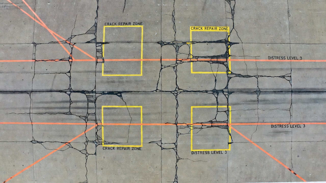
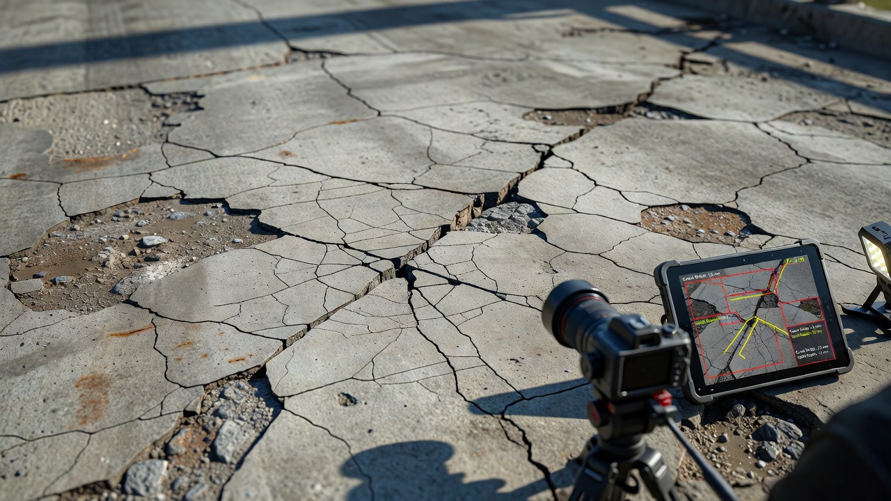
Crack detection — the task of identifying and localizing cracks in infrastructure surfaces — is the most studied application of data augmentation in the infrastructure inspection domain. Cracks present unique challenges that make augmentation particularly impactful.
Cracks in concrete and asphalt surfaces exhibit the following properties relevant to augmentation design:
High aspect ratio — Cracks are long and narrow, with width-to-length ratios often exceeding 1:100. This means geometric augmentations that strongly distort aspect ratios (extreme shear, non-square crops) can make cracks unrecognizable. Linearity preservation — Most structural cracks follow roughly linear or gently curved paths, though alligator cracking forms interconnected polygonal networks. Augmentations that break linear continuity (random erasing of crack center, aggressive JPEG compression) can destroy the crack signature. Low contrast — Fine cracks (hairline cracks under 0.3mm width) have minimal contrast against the surrounding pavement — often only 5-15 gray-level differences on an 8-bit image. Color augmentations must be applied with care to avoid erasing this already weak signal. Texture dependence — Cracks are detected as anomalies against the background pavement texture. Augmentations that homogenize texture (excessive blur, strong equalization) can make cracks indistinguishable from intact pavement.
Based on published research and empirical testing on airfield pavement datasets, the following pipeline is recommended for crack detection models:
Stage 1 — Geometric core: Horizontal flip (50%), random rotation ±45° (30%), random crop to 80-95% with resize (always). These augmentations are always applied because crack orientation and position are nuisance variables.
Stage 2 — Lighting simulation: Color jitter with brightness ±0.3, contrast ±0.3, saturation ±0.2, hue ±0.1 (50% probability). This simulates the full range of operational lighting conditions.
Stage 3 — Quality simulation: Gaussian blur σ=0.5-2.0 (25% probability), Gaussian noise σ=0.01-0.03 (15% probability). This simulates capture quality variation.
Stage 4 — Domain simulation: Shadow overlay with random polygon mask (20% probability), wet surface simulation with increased saturation and specular highlights (15% probability). This simulates field conditions.
Stage 5 — Regularization: Cutout with patch size 16-32 pixels (10% probability). This prevents overfitting to specific image regions.
This pipeline maintains label validity — the crack remains a crack after all transformations — while exposing the model to extreme variability in appearance.
Defect classification — assigning a categorical label to an image patch (e.g., “crack,” “spall,” “weathering,” “intact”) — has different augmentation requirements than pixel-level segmentation.
Infrastructure defect datasets are severely imbalanced by nature. Intact pavement dominates every dataset, while individual defect classes may have only hundreds of examples. Data augmentation addresses this imbalance through class-aware augmentation: applying more aggressive or more numerous transforms to under-represented classes to increase their effective representation in each training batch.
For example, if the training dataset contains 10,000 intact images, 500 crack images, and 200 spall images, the augmentation pipeline can be configured to apply 5 randomly sampled augmentations to each spall image (generating 5×200 = 1,000 effective spall examples per epoch) while applying only 1 augmentation to each intact image. This class-aware augmentation strategy improves classifier sensitivity to rare defect types without requiring additional data collection.
For classification, it is essential that augmentations are label-preserving — the transformed image must still belong to the original class. Some transformations can change the label:
For classification, the augmentation magnitude must be calibrated to the minimum detectable feature size of each defect class. For hairline cracks (minimum width ~0.2mm at the capture resolution), blur exceeding σ=2.0 and rotations beyond ±60° should be applied with reduced probability or excluded.
Infrastructure surfaces often exhibit multiple concurrent defect types — a spalled area may contain cracks, or a weathered patch may have joint sealant failure. For multi-label classification, augmentation must be consistent across all labels for a given image. The same geometric transform applied to the image applies to all labels simultaneously. Color and noise transforms are inherently label-preserving for multi-label classification because they don’t change the presence or absence of any defect type.
The relationship between data augmentation and overfitting is fundamental to understanding augmentation’s role in deep learning.
Overfitting occurs when a model with high capacity (many trainable parameters) is trained on a dataset with insufficient size or diversity. The model learns not the general patterns of the defect class but the specific pixel arrangements, textures, and artifacts of the training examples. Mathematically, overfitting manifests as the model learning a degenerate mapping from input to output that minimizes training loss but fails to minimize expected loss on the true data distribution.
For infrastructure inspection models, overfitting typically appears after 50-100 training epochs. Training accuracy continues to rise toward 100 percent while validation accuracy plateaus and then declines. The gap between training and validation accuracy — the generalization gap — widens progressively. Without augmentation, a ResNet-50 trained on 2,000 crack images will typically show a 15-25 percent generalization gap. With comprehensive augmentation, this gap can be reduced to 3-5 percent or less.
The key mechanism by which augmentation prevents overfitting is increasing the effective training set size. With on-the-fly augmentation applied during training, each image is transformed differently at each epoch. A training dataset of 5,000 images with an augmentation policy that applies 3 random transforms from a pool of 10 operations, each with 5 possible magnitudes, generates 5,000 × 10³ × 5³ ≈ 6.25 million distinct training examples over 100 epochs.
This effective dataset expansion is particularly valuable for infrastructure inspection because:
Data augmentation functions as a regularizer in the statistical learning sense. By expanding the training distribution, augmentation reduces the model’s ability to fit noise in the original dataset. The variance of the learned parameters decreases because the model must satisfy constraints from many more effectively independent training examples.
The regularization strength of augmentation is controlled by:
For infrastructure inspection models, the optimal regularization-augmentation balance is found by monitoring the validation loss trajectory. If validation loss increases while training loss continues decreasing (overfitting), augmentation magnitude or probability should be increased. If both training and validation loss are high (underfitting), augmentation should be reduced to allow the model to learn more from the raw training data.
Implementing data augmentation in a production training pipeline requires careful architectural decisions about when, where, and how augmentations are applied.
Offline augmentation pre-generates augmented images and saves them to disk before training begins. The augmented dataset might contain 50,000 images derived from 5,000 originals through 10 fixed augmentations per image. Training then proceeds on this fixed augmented dataset.
Online augmentation applies transformations on-the-fly during training, with each image loaded from disk, randomly augmented, and fed to the model immediately. No augmented images are permanently stored.
Online augmentation is the standard approach for production infrastructure inspection pipelines because:
The computational cost of online augmentation is minimal — modern GPU-accelerated augmentation libraries (NVIDIA DALI, Kornia, or PyTorch’s torchvision) apply transformations in microseconds per image, typically representing less than 5 percent of total training time when data loading is pipelined with GPU execution.
The choice of augmentation library impacts pipeline performance, flexibility, and maintainability:
Albumentations is the most widely used library for infrastructure inspection due to its speed (optimized C++ backend via OpenCV), comprehensive operation set (70+ transforms), and native dual-channel augmentation support for segmentation masks. Albumentations ensures that any geometric transform applied to the image is identically applied to the mask, maintaining pixel-level alignment between input and ground truth.
NVIDIA DALI provides GPU-accelerated data loading and augmentation pipelines that can process images entirely on the GPU, avoiding CPU-GPU transfer bottlenecks. DALI is recommended for very large training datasets (10,000+ images) where data loading time dominates training time.
torchvision.transforms (PyTorch) and tf.image (TensorFlow) provide built-in augmentation capabilities with good integration with their respective frameworks but have fewer domain-specific transforms (shadow simulation, perspective, random erasing) than Albumentations.
In a production training pipeline, augmentation is integrated as follows:
[Image Loader] → [Random Sampler] → [Augmentation Sequence] → [Normalize] → [Random Batch Sampler] → [Model Forward Pass]
The random sampler selects whether each augmentation in the policy is applied (based on its probability parameter) and the magnitude each time. The augmentation sequence applies transforms in a fixed order: typically geometric first (crop, flip, rotate, perspective), then photometric (color jitter, brightness, contrast), then noise and blur (Gaussian noise, Gaussian blur), then domain-specific (shadow, rain), and finally regularization (Cutout).
During validation and inference, augmentation is reduced to the minimum necessary transforms: typically only center-crop (or resize) and normalization. No random transforms are applied during evaluation to ensure deterministic, reproducible results.
Production training pipelines should log augmentation statistics to monitor their effect on training dynamics:
These monitoring metrics ensure that augmentation is achieving its intended effect — expanding the training distribution without introducing artifacts or biases that degrade real-world performance.
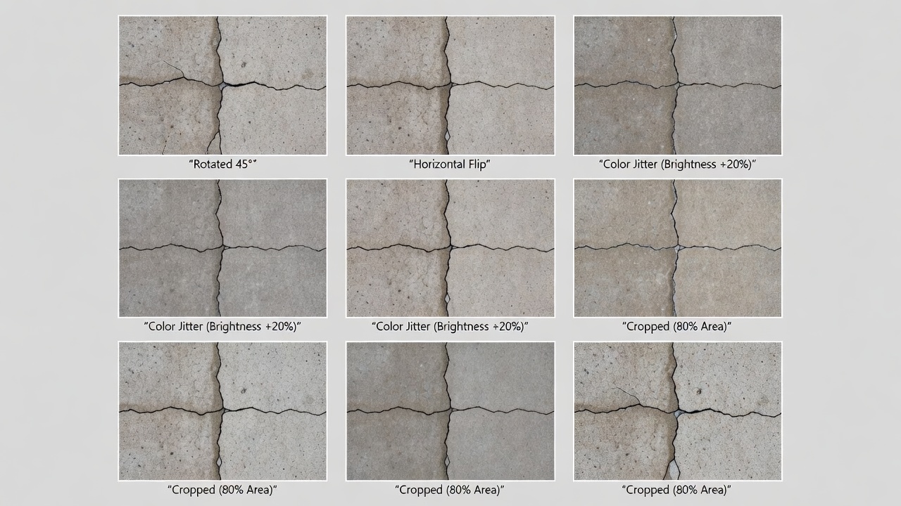
The image show of concrete crack grid augmentations demonstrates the practical output of an augmentation pipeline: the same original crack image is transformed into 12+ distinct training examples through rotation, flipping, cropping, color adjustment, and blur. Each augmented version preserves the crack label while presenting it in a visually different context, teaching the model to detect cracks regardless of orientation, lighting, or image quality.
{
TarmacView leverages advanced data augmentation pipelines to train infrastructure inspection models that generalize across lighting, weather, and surface conditions. Optimize your defect detection model training with domain-specific augmentation strategies tailored for airfield pavements and concrete structures.
Transfer learning applies knowledge from a model pre-trained on large general datasets (ImageNet 1.2M images, DINOv3 on 1.7B images) to specialized infrastructu...
Domain adaptation adapts machine learning models trained on a source domain — such as specific pavement types, lighting conditions, or datasets — to perform rel...
AI-based crack detection uses computer vision — convolutional neural networks, vision transformers, and semantic segmentation models — to automatically identify...