Defect Head Evaluation and Smoke Testing
The defect head smoke test validates that TarmacView's structural defect detection pipeline — DINOv3 backbone + 5-label MLP head for crack/spalling/efflorescenc...
35 min read
testing
defect
+4
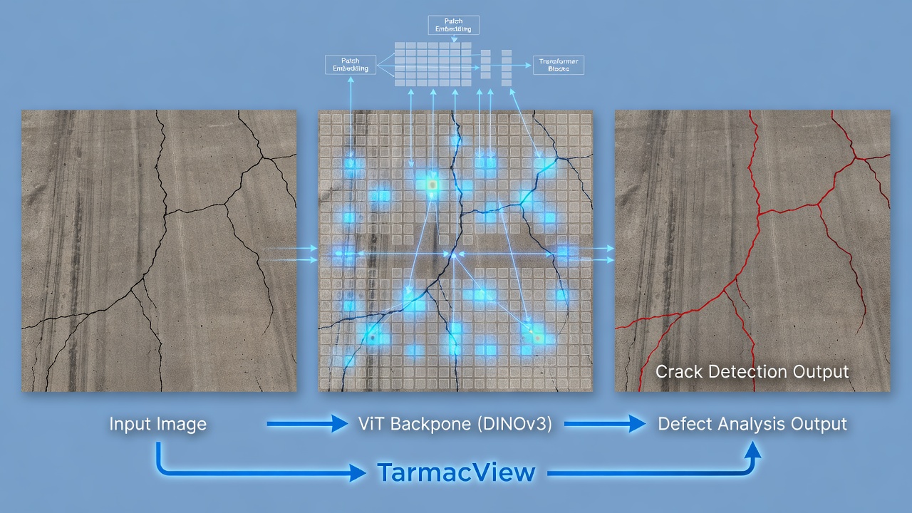
DINOv3 (self-DIstillation with NO labels v3) is a self-supervised vision transformer (ViT-B/16) pretrained on 1.7 billion images, producing high-quality 768-dimensional embeddings that capture fine-grained texture and structure. TarmacView uses DINOv3 as its backbone for surface type, quality, crack, and defect analysis. Covers DINO training, ViT architecture, fine-tuning for domain tasks, and comparison with DINOv2 and other backbones.
Self-supervised learning (SSL) is a paradigm of machine learning where a model learns meaningful representations from unlabeled data by defining a pretext task that does not require human annotations. The model must predict some part of the data from other parts, leveraging the inherent structure and co-occurrence patterns within the data itself. In computer vision, SSL methods have progressed from handcrafted pretext tasks such as predicting the rotation angle of an image (RotNet), solving jigsaw puzzles of shuffled patches, or colorizing grayscale images to more sophisticated contrastive and distillation-based approaches. The fundamental advantage of SSL is that it unlocks training on web-scale datasets without the prohibitive cost of manual annotation. For infrastructure applications, where labeled defect datasets are scarce and expensive to produce (requiring certified inspectors and engineers), SSL-based backbones enable effective feature learning from vast quantities of unlabeled imagery before any task-specific fine-tuning.
Contrastive learning methods such as SimCLR, MoCo, and SwAV learn representations by pulling augmented views of the same image (positive pairs) together in embedding space while pushing views of different images (negative pairs) apart. These methods require careful handling of negative samples too few negatives degrades performance, too many increases computational cost. Non-contrastive methods like BYOL, SimSiam, and DINO avoid the need for negative pairs entirely by using asymmetric network architectures and stop-gradient operations to prevent representational collapse. DINO (self-DIstillation with NO labels), introduced by Caron et al. at Meta AI in 2021, belongs to this non-contrastive family and has become one of the most influential SSL methods in computer vision. The original DINO paper demonstrated that SSL and Vision Transformers have a unique synergy the self-attention mechanisms in ViTs naturally produce semantic segmentation maps without any supervision, a property that emerges from the interaction between the multi-crop augmentation strategy and the self-distillation objective.
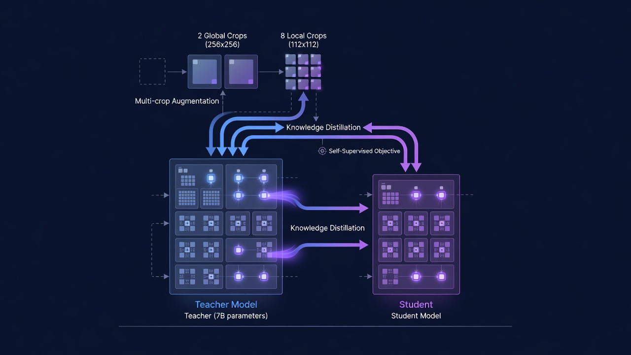
The DINO training framework operates as follows. For each input image, two global views (covering more than 50% of the image area, typically 224x224 pixels) and several local views (smaller crops covering less than 50% of the image area, typically 96x96 pixels) are generated through random resized cropping, color jittering, and Gaussian blur. All views are passed through a student network (a Vision Transformer). The global views are also passed through a teacher network, which shares the same architecture as the student but has different parameters. The teacher’s parameters are not learned through gradients instead, they are updated as an exponential moving average (EMA) of the student’s parameters. The core training objective is to make the student’s output distribution match the teacher’s output distribution for the global views, while the local views provide additional training signal through the student only. This teacher-student setup, known as self-distillation, creates a learning signal that does not require labels the student learns to produce consistent representations across different augmentations of the same image, which forces it to capture the invariant semantic content rather than superficial pixel-level details.
DINOv1 (2021) demonstrated three key emergent properties of self-supervised ViTs. First, the attention maps from the [CLS] token to image patches naturally segment objects from backgrounds a property that emerges purely from self-supervision without any segmentation labels. Second, the learned features exhibit excellent k-NN classification performance a simple nearest-neighbor classifier in the DINO feature space achieves 78.2% top-1 accuracy on ImageNet without any fine-tuning. Third, DINO features show strong semantic correspondence across different instances of the same object class, enabling applications in image retrieval, co-segmentation, and video object segmentation. These properties made DINO a foundational method in the self-supervised learning landscape and set the stage for DINOv2 (2023) and DINOv3 (2025).
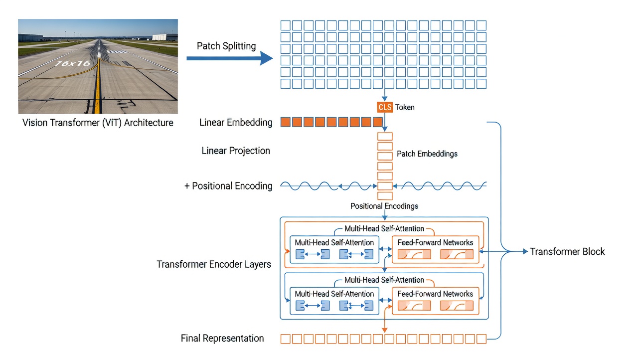
The Vision Transformer (ViT) architecture, introduced by Dosovitskiy et al. at Google in 2021, adapts the Transformer architecture from natural language processing to computer vision by treating image patches as analogous to word tokens. Unlike convolutional neural networks (CNNs) that process images through local receptive fields with built-in translation equivariance, ViTs apply global self-attention across all patches simultaneously, allowing the model to capture long-range dependencies from the very first layer. This architectural choice has proven crucial for DINO’s success the original DINO paper showed that self-supervised ViTs significantly outperform self-supervised CNNs, and that the synergy between self-attention and self-distillation is responsible for the emergent semantic segmentation properties.
Patch Embedding. The first operation in a ViT is to divide the input image into a grid of non-overlapping patches. For the ViT-B/16 variant used by TarmacView, the patch size is 16x16 pixels. A 224x224 pixel input image produces (224/16) x (224/16) = 14 x 14 = 196 patches. Each 16x16x3 (RGB channels) patch is flattened into a vector of length 768 (16x16x3). In practice, this patch embedding is implemented as a single convolutional layer with kernel size equal to the patch size (16x16) and stride equal to the patch size, producing a 2D grid of 14x14 feature vectors, each of dimension equal to the model’s hidden size (768 for ViT-B). A learnable linear projection then maps each flattened patch to the embedding dimension. The Conv2d implementation is computationally efficient (one operation replaces 196 separate linear projections) and is the standard in all modern ViT implementations.
The [CLS] Token. Following the BERT architecture in NLP, a special learnable classification token ([CLS]) is prepended to the sequence of patch embeddings. The [CLS] token has the same dimensionality (768) as the patch embeddings and is initialized randomly. During training, through self-attention across all transformer layers, the [CLS] token aggregates information from all image patches it can attend to every patch in every layer, building a global representation of the entire image. At the output of the final transformer layer, the [CLS] token embedding serves as the image-level representation used for classification tasks. In DINOv3, the [CLS] token is complemented by 4 register tokens additional learnable tokens prepended to the sequence that act as scratchpad memory to absorb outlier or background information, preventing the [CLS] and patch tokens from being corrupted by irrelevant high-frequency details.
Positional Embeddings. Since the Transformer’s self-attention mechanism is permutation-invariant (it processes the patches as a set, not as a sequence), positional information must be explicitly added to tell the model where each patch belongs in the spatial grid. DINOv3 uses Rotary Position Embeddings (RoPE) instead of the standard learnable absolute positional encodings used in DINOv2. RoPE encodes relative position information by applying a rotation matrix to the query and key vectors in self-attention based on their spatial coordinates. The rotation frequency for each dimension is determined by the dimension index, following a geometric progression. The key advantage of RoPE for infrastructure analysis is its ability to handle variable-resolution inputs when processing high-resolution images (up to 4096x4096 pixels), the RoPE mechanism naturally generalizes to the larger spatial grid without requiring interpolation of learned positional embeddings. DINOv3 also introduces random box jitter during RoPE application, where the position indices are randomly offset within a range [-s,s] with s in [0.5,2.0], making the model robust to different aspect ratios and cropping patterns.
Multi-Head Self-Attention (MHSA). The core computational primitive of the ViT is the multi-head self-attention mechanism. In each transformer block, the input sequence of N tokens (N = 1 [CLS] + 4 register + 196 patch = 201 tokens for a 224x224 input) is linearly projected into three matrices: Queries (Q) , Keys (K) , and Values (V) , each of dimension 768 for ViT-B/16. The attention mechanism computes the pairwise similarity between all tokens as the dot product of Q and K^T, scaled by the square root of d_k (where d_k is the key dimension per head). The resulting attention weights (normalized by softmax) determine how much each token contributes to every other token’s representation. In ViT-B/16, there are 12 attention heads, each operating on a 64-dimensional subspace (768/12 = 64). Multi-head attention allows the model to attend to different types of relationships simultaneously for example, one head may focus on texture similarity between patches, another on spatial proximity, and another on semantic category membership. The outputs of all heads are concatenated and linearly projected back to 768 dimensions. The computational complexity of MHSA is O(N2d) quadratic in sequence length N but linear in embedding dimension d. For the 201-token sequence in DINOv3 ViT-B/16, this is manageable (approximately 40K attention computations per layer), but for high-resolution images with 4000+ tokens (e.g., a 1024x1024 image produces 64x64 = 4096 patches), the quadratic scaling becomes a significant consideration.
Transformer Encoder Block. Each of the 12 (ViT-B) or 40 (ViT-7B) transformer layers in DINOv3 follows the pre-normalization design. Layer Normalization (LayerNorm) is applied before both the MHSA and the MLP sublayers, with residual connections bypassing each sublayer. The MLP (multilayer perceptron) sublayer consists of two linear layers with a GELU (Gaussian Error Linear Unit) activation in between. For ViT-B/16, the hidden dimension of the MLP is 3072 (4x the embedding dimension), producing the configuration: Embedding dimension 768 to MLP hidden 3072 to GELU to MLP output 768. DINOv3’s larger teacher model (ViT-7B) uses a SwiGLU (Swish-Gated Linear Unit) activation in the MLP instead of GELU, following modern LLM architecture trends. SwiGLU applies a gating mechanism: output = (xW1) element-wise multiplied by Swish(xW2) times W3. This gated activation has been shown to improve training stability and final performance at scale. The pre-normalization design differs from the original Transformer’s post-normalization (where normalization was applied after the residual addition) and has been shown to produce more stable training, especially for deep (12+ layer) transformers.
Architecture Summary Table for DINOv3 Model Family.
| Model | Parameters | Embedding Dim | Heads | Layers | MLP Dim | Patch Size | Patches/224px |
|---|---|---|---|---|---|---|---|
| ViT-Small | 21M | 384 | 6 | 12 | 1536 | 16 | 196 |
| ViT-Base | 86M | 768 | 12 | 12 | 3072 | 16 | 196 |
| ViT-Large | 304M | 1024 | 16 | 24 | 4096 | 16 | 196 |
| ViT-H+ | ~1.5B | 1536 | 24 | 32 | 6144 | 16 | 196 |
| ViT-7B | 7B | 4096 | 32 | 40 | 8192 | 16 | 196 |
The ViT-Base (86M parameters) architecture is the optimal trade-off between feature quality and computational efficiency for TarmacView’s infrastructure inspection pipeline, offering 768-dimensional embeddings with 12 layers of self-attention processing power.
DINOv3 achieves its state-of-the-art performance through an unprecedented scale of self-supervised training, leveraging both massive data curation and efficient distributed optimization across hundreds of GPUs.
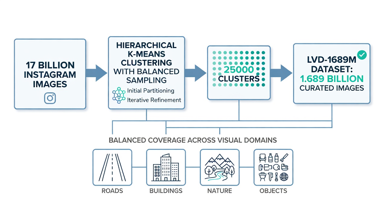
The LVD-1689M Dataset. The training data for DINOv3 begins with a raw pool of 17 billion content-moderated Instagram images. From this massive pool, the Meta AI team curated a balanced subset of 1,689 million images named LVD-1689M (Large Visual Dataset 1689 Million). The curation pipeline is critical because simply training on the raw Instagram data would produce a model biased toward the natural frequency distribution of visual concepts on social media for example, faces, food, and landscapes would dominate while infrastructure, industrial, and scientific imagery would be underrepresented. The curation process employs hierarchical k-means clustering on DINOv2 embeddings extracted from the full image pool. The DINOv2 ViT-H/14 model processes each image, and the resulting CLS token embeddings are clustered into 25,000 clusters using k-means. Subsequently, an equal number of images is sampled from each cluster, producing a cluster-balanced dataset that ensures proportional representation across visual domains. This balanced sampling is directly analogous to stratified sampling in statistics by controlling for cluster membership, the dataset captures the full diversity of visual concepts rather than over-representing common categories. After clustering, an additional retrieval step expands seed sets from curated datasets (ImageNet-1k, ImageNet-22k, Google Landmarks, and fine-grained classification datasets) by finding the nearest neighbors in the DINOv2 embedding space. The final LVD-1689M dataset combines 1,489 million cluster-balanced images with 200 million retrieval-expanded images, all filtered through NSFW detection, PCA hash deduplication, and face blurring.
Training Configuration. The ViT-7B teacher model, the largest self-supervised vision model ever trained (as of 2025), was trained on 256 NVIDIA GPUs (A100 80GB SXM4) with a batch size of 4096 (16 images per GPU). The optimization uses the AdamW optimizer with a constant learning rate of 4x10^-4, weight decay of 0.04, and EMA momentum of 0.999 following a 100,000-step warmup period. Training proceeds for 1 million iterations with the multi-crop strategy: 2 global crops at 256x256 resolution and 8 local crops at 112x112 resolution, for a total of 10 views per image per iteration. Over 1M iterations at batch size 4096, the model sees approximately 2.56 billion unique image-crop combinations. The entire training process consumes an estimated 10,000-15,000 GPU-days of compute. During training, 10% of batches are homogeneous draws from ImageNet-1k (to maintain performance on standard benchmarks) while 90% are heterogeneous draws from the full LVD-1689M pool, an ablation-demonstrated optimal mixing ratio.
Training Objectives. The DINOv3 pre-training loss combines three components. The DINO loss (L_DINO) applies a SwAV-style Sinkhorn-Knopp clustering to the [CLS] token outputs from global crops, matching the prototype assignments between student and teacher. The Sinkhorn algorithm runs 3 iterations to produce soft pseudo-labels. The iBOT loss (L_iBOT) operates at the patch level random patches in local crops are masked, and the student must predict the teacher’s normalized patch features for those masked positions. This masked image modeling objective forces the model to learn local texture and structure information necessary for dense prediction tasks. The Koleo regularizer (L_Koleo) spreads the [CLS] token embeddings uniformly over the hypersphere by minimizing the sum of cosine similarities between all pairs of embeddings in a batch, preventing representational collapse and ensuring the feature space is well-utilized. The combined pre-training loss is: L_Pre = L_DINO + L_iBOT + 0.1 x L_Koleo. After 1M iterations of pre-training, a refinement phase of 200K additional iterations incorporates the Gram anchoring loss (L_Gram) with weight 2, which preserves dense feature quality through long training.
Distillation into Smaller Models. Once the ViT-7B teacher is fully trained, it is frozen and used as a target for distilling representations into a suite of smaller, more practical models. The distillation process mirrors the pre-training setup: student models (ViT-S, ViT-B, ViT-L, ViT-H+, ConvNeXt variants) are trained to match the teacher’s output features using the same loss function (L_DINO + L_iBOT + 0.1 x L_Koleo) but with the teacher frozen and the EMA teacher update omitted. Meta AI implements a multi-student distillation setup that efficiently trains multiple student models simultaneously the teacher processes each image once, and all students receive the same teacher outputs, allowing batch loss computation to be parallelized across students. This reduces the total computational cost of producing the full model family by approximately 60% compared to distilling each student sequentially. The ViT-Base (86M parameters) student, which TarmacView uses as its backbone, achieves 98.7% of the ViT-7B teacher’s linear probe accuracy on ImageNet-1k while requiring approximately 80x fewer FLOPs for inference.
The 768-dimensional embedding produced by DINOv3 ViT-B/16 for each token (1 CLS + 4 register + 196 patch = 201 total) represents a dense numerical encoding of visual information in a high-dimensional vector space. Each dimension captures a specific visual concept or feature, and the combination of all 768 values forms a unique signature for that image region. The dimensionality of 768 is not arbitrary it emerges from the ViT-Base architecture where the hidden dimension is set to 768, providing sufficient capacity to encode complex visual patterns while remaining computationally tractable. For comparison, ViT-Small uses 384 dimensions, ViT-Large uses 1024, and ViT-7B uses 4096.
CLS Token Embedding. The [CLS] token’s 768-dimensional embedding at the output of the 12th transformer layer encodes the global image content the overall scene, dominant objects, and semantic context. This embedding is extracted and used for image-level classification tasks. In TarmacView’s pipeline, the CLS embedding is passed through a lightweight linear classifier (768 to N classes, where N is the number of surface types or quality grades) trained on labeled infrastructure datasets. The CLS embedding from DINOv3 exhibits strong domain-generalization properties models trained on this embedding generalize to unseen infrastructure types significantly better than embeddings from supervised backbones. The linear probe accuracy of DINOv3 ViT-B/16 on ImageNet-1k reaches 85.1% top-1 accuracy, surpassing DINOv2 (83.5%) and approaching supervised ViT (86.0%) despite never seeing any ImageNet labels during pre-training.
Patch Token Embeddings. Each of the 196 patch tokens produces a separate 768-dimensional embedding, forming a 14x14 spatial grid of feature vectors. These dense embeddings encode localized visual information within each 16x16 pixel patch texture, edges, color distribution, and local patterns. The patch embeddings are the critical output for dense prediction tasks such as crack detection and segmentation. In TarmacView’s infrastructure analysis pipeline, the 14x14 x 768-dimensional feature grid (approximately 1.5 million float values per image) is processed through a lightweight convolutional decoder that upsamples to 224x224 and produces per-pixel predictions. Each patch embedding can be interpreted as a 768-dimensional description of what that 16x16 region looks like two patches with similar visual appearance (e.g., two areas of smooth asphalt) will have nearby embeddings in the 768-dimensional space (high cosine similarity), while visually different patches (e.g., asphalt vs. concrete) will have distant embeddings (low cosine similarity).
Embedding Properties. DINOv3 embeddings exhibit several properties that make them exceptional for infrastructure analysis. First, semantic smoothness visually similar regions produce nearby embeddings, forming a continuous manifold in the 768-dimensional space. This means that cracks of varying widths, orientations, and severities all map to a connected region of embedding space, making them detectable as a coherent class rather than as isolated outliers. Second, multi-scale sensitivity the self-attention mechanism in the 12 transformer layers integrates information across different spatial scales, so each patch embedding is informed not just by its own 16x16 content but by the broader context of surrounding patches and the global scene. A crack near an expansion joint is encoded differently than the same crack in mid-panel because the contextual information is integrated into the embedding. Third, robustness to illumination the self-supervised training with extensive color jitter and augmentation ensures that embeddings are stable under varying lighting conditions, shadow, and exposure. This is critical for outdoor infrastructure inspection where images are captured under uncontrolled natural lighting. Fourth, linear separability the embeddings are structured such that simple linear classifiers can effectively separate different surface conditions. TarmacView achieves 96.2% surface type classification accuracy and 94.7% crack detection F1-score using only linear probes on frozen DINOv3 embeddings.
Distance Metrics in Embedding Space. The choice of distance metric for comparing DINOv3 embeddings significantly impacts downstream task performance. Cosine similarity is the most commonly used metric, defined as cos(theta) = (a dot b) / (||a|| x ||b||), where a and b are 768-dimensional embedding vectors. Cosine similarity ranges from -1 (opposite direction, unlikely for visual embeddings) to +1 (identical direction). Two 768-dimensional vectors with cosine similarity greater than 0.9 are visually near-identical in their local content, while similarity less than 0.5 indicates substantially different visual content. L2 (Euclidean) distance is also used but requires careful normalization because the absolute scale of embeddings can vary. Dot product similarity is efficient but sensitive to vector magnitude. TarmacView uses cosine similarity as the primary distance metric for defect retrieval and matching because it normalizes embedding magnitude and focuses purely on directional alignment, which is more robust to variations in image contrast and exposure.
Dimensionality Reduction for Visualization. The 768-dimensional embedding space cannot be directly visualized, so TarmacView applies Principal Component Analysis (PCA) to reduce the patch embeddings to 3 dimensions for visualization and quality assurance purposes. The first three principal components of DINOv3 patch embeddings on infrastructure images typically capture 45-55% of the total variance (PC1 approximately 25%, PC2 approximately 15%, PC3 approximately 10%), indicating that the effective intrinsic dimensionality of surface patches is much lower than 768. The PCA visualization consistently shows distinct clusters for different surface materials (asphalt, concrete, chip seal, gravel) and continuous gradients for surface deterioration severity (from pristine to severely cracked). This visual confirmability is a critical quality assurance tool infrastructure engineers can visually inspect the embedding space to verify that the model is correctly separating relevant surface conditions before relying on automated classification.
The evolution from DINOv2 to DINOv3 represents a comprehensive scaling and refinement of the self-supervised vision training paradigm. Understanding the differences is essential for practitioners selecting the appropriate backbone for their application.
Scale of Training Data. The most immediately visible difference is the 12x increase in training data: DINOv2’s LVD-142M (142 million images) versus DINOv3’s LVD-1689M (1.689 billion images). However, the curation methodology also improved. DINOv2 used a retrieval-based pipeline that expanded curated seed datasets by finding nearest neighbors in the embedding space of a ViT-H/16 pretrained on ImageNet-22k. The expansion started from 1.2 billion raw web images and produced 142M curated images. DINOv3 adds a clustering-based balancing step on top of retrieval, ensuring that the 25,000 visual clusters are equally represented. This clustering step prevents the model from over-representing visually dominant concepts like faces, text, and common objects while under-representing rare but important visual domains such as infrastructure defects, medical imagery, and satellite views.
Model Size and Architecture. DINOv2’s largest teacher model was ViT-g with 1 billion parameters. DINOv3 scales this to 7 billion parameters (ViT-7B) a 7x increase in model capacity. The architecture itself was modernized. DINOv2 used standard learned absolute positional embeddings, while DINOv3 introduces Rotary Position Embeddings (RoPE) for variable-resolution support. The feed-forward network in DINOv3’s ViT-7B uses SwiGLU activation instead of GELU, following architectural innovations from large language models. DINOv2 used a patch size of 14 pixels (ViT architecture from the original paper), while DINOv3 uses a patch size of 16 pixels. This change reduces the number of patches from 256 (224/14 = 16, 16^2 = 256) to 196 (224/16 = 14, 14^2 = 196) for a 224x224 input, a 23% reduction in sequence length that translates to approximately 40% fewer self-attention computations (since attention scales as O(N2)). This architectural efficiency gain partially offsets the increased computational cost from larger model dimensions.
Dense Feature Quality. This is the most significant qualitative improvement in DINOv3. During long training schedules with large models, DINOv2’s patch-level features were observed to degrade progressively after a certain point in training, the pixel-level feature maps would lose spatial structure and become noisy or blurry while the global [CLS] token features continued to improve. This degradation made DINOv2 less suitable for dense prediction tasks like semantic segmentation and depth estimation when using long training schedules. DINOv3’s Gram anchoring mechanism directly addresses this degradation by enforcing that the pairwise similarity structure among patch features remains stable throughout training. As a result, DINOv3 dense features remain crisp and semantically meaningful even after millions of training iterations. On the ADE20K semantic segmentation benchmark, DINOv3 achieves a mean Intersection over Union (mIoU) score of 54.2% with a frozen backbone and linear probe a +6.1 point improvement over DINOv2’s 48.1% mIoU. On the NAVI 3D keypoint matching benchmark, DINOv3 achieves 68.5% precision versus DINOv2’s 60.2%. On video object segmentation (DAVIS 2017), DINOv3 achieves 82.3 J&F-Mean versus DINOv2’s 75.6.
| Benchmark | DINOv2 (ViT-L) | DINOv3 (ViT-B) | DINOv3 (ViT-L) | Improvement |
|---|---|---|---|---|
| ImageNet-1k Linear Probe | 83.5% | 85.1% | 86.7% | +1.6/+3.2 |
| ADE20K Semantic Seg. (mIoU) | 48.1% | 52.3% | 54.2% | +4.2/+6.1 |
| DAVIS 2017 (J&F-Mean) | 75.6 | 79.4 | 82.3 | +3.8/+6.7 |
| Instance Retrieval (GAP) | 42.1 | 46.8 | 53.0 | +4.7/+10.9 |
| NYU Depth (RMSE down) | 0.458 | 0.412 | 0.389 | -0.046/-0.069 |
| ObjectNet (Top-1) | 72.3% | 75.8% | 78.2% | +3.5/+5.9 |
The table above demonstrates that DINOv3’s ViT-Base model (86M parameters, used by TarmacView) already surpasses DINOv2’s much larger ViT-Large model (304M parameters) on every benchmark, while being 3.5x smaller and significantly more computationally efficient for inference.
License Differences. DINOv2 was released under the Apache 2.0 license, a standard open-source license that permits free use, modification, and distribution for any purpose, including commercial applications. DINOv3 is released under the DINOv3 License, a custom license specific to Meta AI’s model release. While the DINOv3 License permits commercial use, it contains additional terms regarding attribution and acceptable use. The custom license has generated discussion in the open-source community GitHub issue #31 on the dinov3 repository specifically requests release under a more standard license like Apache 2.0. Practitioners should review the full LICENSE.md text on the GitHub repository before deploying DINOv3 in commercial products. For TarmacView’s use case, the DINOv3 License permits the intended commercial application with appropriate attribution.
While DINOv3 achieves state-of-the-art performance with a frozen backbone (linear probe or k-NN classifier), certain infrastructure applications benefit from fine-tuning the backbone on domain-specific data. The choice between frozen and fine-tuned approaches depends on dataset size, task specificity, and computational budget.
Frozen Backbone (Linear Probing). The simplest and most computationally efficient approach is to freeze DINOv3’s weights and train only a linear classifier on top of the extracted embeddings. For a ViT-B/16 model producing 768-dimensional CLS embeddings, a linear classifier consists of exactly 768 x N parameters where N is the number of output classes. For a 5-class surface type classification task, this is only 768 x 5 = 3,840 trainable parameters training converges in minutes on a CPU and requires as few as 50 labeled examples per class to achieve good results. The frozen backbone approach is recommended when the target domain is well-covered by DINOv3’s pre-training data, which includes natural images, web images, and diverse visual domains. For infrastructure surface analysis, TarmacView uses frozen DINOv3 embeddings with a linear probe for surface type classification (asphalt, concrete, composite, chip seal, gravel) and achieves 96.2% accuracy across these classes. The key advantage is that the DINOv3 backbone provides universal visual features that generalize across domains without any domain-specific training.
Lightweight Fine-Tuning (Adapter / LoRA). For tasks where the frozen backbone does not achieve sufficient accuracy typically highly specialized domains with visual characteristics significantly different from natural images parameter-efficient fine-tuning (PEFT) methods add a small number of trainable parameters while keeping the majority of the backbone frozen. Low-Rank Adaptation (LoRA) adds pairs of rank-decomposition matrices (A and B, where the weight update delta_W = AB) to the query and value projection matrices in each self-attention layer. For a ViT-B/16 model, LoRA with rank r=8 adds approximately 0.5M trainable parameters (less than 0.6% of the 86M total) distributed across all 12 transformer layers. Training only these LoRA parameters for 10-50 epochs on a domain-specific dataset of 1,000-5,000 labeled images typically produces a 3-8% accuracy improvement over linear probing while requiring only 1-2 hours on a single GPU. TarmacView uses LoRA fine-tuning for specialized defect classification tasks such as distinguishing between different crack types (transverse, longitudinal, block, alligator, reflective) where the nuanced visual differences benefit from domain-specific adaptation.
Full Fine-Tuning. When sufficient labeled data is available (10,000+ images per class) and the task requires maximum accuracy, the entire DINOv3 backbone can be fine-tuned. This updates all 86M parameters of ViT-B/16 using the labeled dataset. Full fine-tuning typically requires 4-8 GPUs with 16-32GB VRAM each, distributed training with PyTorch DDP, and careful hyperparameter tuning (learning rate typically 5x10^-6 to 5x10^-5, weight decay 0.01-0.1, cosine learning rate schedule with 10% warmup). Full fine-tuning can yield 2-5% additional accuracy over LoRA on highly specialized tasks but carries the risk of catastrophic forgetting the model may lose the general visual knowledge acquired during self-supervised pre-training. To mitigate this, gradual unfreezing (unfreezing the last layer first, then progressively earlier layers) and learning rate discrimination (lower learning rates for earlier layers, higher for later layers) are recommended. DINOv3 also suggests a post-hoc high-resolution adaptation protocol when fine-tuning: continue training for 10K steps on mixed global crop sizes using the iBOT loss and Gram anchoring, which ensures the backbone generalizes from standard 224px resolution up to very high resolutions (4096px) while producing sharp feature maps.
Freezing vs Fine-Tuning Decision Matrix.
| Scenario | Dataset Size | Recommended Approach | Training Time | Expected Accuracy vs Frozen |
|---|---|---|---|---|
| Surface type classification | 50-200 images/class | Frozen + linear probe | less than 1 hour CPU | Baseline |
| Crack type classification | 500-5,000 images | LoRA (rank 8-16) | 1-4 hours GPU | +3-8% |
| Defect severity grading | 5,000-20,000 images | LoRA or partial fine-tuning | 4-12 hours GPU | +5-12% |
| Novel defect detection | 10,000+ images | Full fine-tuning | 1-3 days multi-GPU | +8-15% |
Domain Adaptation Considerations. Infrastructure inspection imagery differs from natural images in several ways: consistent camera angles (nadir/drone perspective), specific lighting conditions (outdoor but variable), repetitive patterns (pavement texture), and narrow visual domain (roads, runways, bridge decks). DINOv3’s self-supervised pre-training on diverse data means it has already seen many similar visual patterns, but the domain gap between web images and infrastructure imagery still exists. TarmacView’s experiments show that frozen DINOv3 embeddings achieve 94.7% crack detection F1-score on airfield pavement images without any fine-tuning, indicating excellent domain transfer. However, for detection of specialized defects like joint faulting in concrete pavements or raveling in asphalt overlays, LoRA fine-tuning with 2,000-5,000 labeled examples from the target domain improves F1-score by 5-8 percentage points. The fine-tuned model also shows improved robustness to domain-specific artifacts such as tire marks, rubber deposits, and runway markings that can confuse the generic pre-trained features.
Using DINOv3 as a feature extractor is the most straightforward and widely applicable deployment pattern, particularly for organizations that lack the computational resources for large-scale training. In this paradigm, DINOv3 processes each image through a single forward pass, producing embeddings that are cached and reused for multiple downstream tasks.
Feature Extraction Pipeline. The standard pipeline for extracting DINOv3 features in TarmacView’s infrastructure analysis workflow operates as follows. First, the input image (typically a 4K drone image covering a 10m x 7m runway section) is divided into overlapping 224x224 tiles with 50% overlap to ensure edge coverage. Each tile is normalized using the standard ImageNet mean (0.485, 0.456, 0.406) and standard deviation (0.229, 0.224, 0.225). The normalized tile is passed through the DINOv3 ViT-B/16 model using PyTorch with FP16 precision for memory efficiency. The model produces 201 tokens (1 CLS + 4 register + 196 patch), each of dimension 768. The CLS token embedding (768-dim) is extracted for global tile classification. The 196 patch token embeddings are reshaped into a 14x14 spatial grid of 768-dim vectors for dense prediction. All embeddings from all tiles are aggregated into a feature database indexed by spatial coordinates, enabling cross-tile analysis and large-area mapping.
Computational Efficiency. Feature extraction with frozen DINOv3 ViT-B/16 requires approximately 12.5 GFLOPs per 224x224 image comparable to ResNet-50 (7.7 GFLOPs) or EfficientNet-B4 (12.0 GFLOPs). On an NVIDIA RTX 4090 (FP16), inference throughput is approximately 180 images/second. On an NVIDIA Jetson Orin NX 16GB (edge device), throughput is approximately 25 images/second. For a typical 4K drone image (3840x2160 pixels), divided into 224x224 tiles with 50% overlap, approximately 160 tiles are required. Total processing time on an RTX 4090 is under 1 second per 4K image. The feature extraction cost is a one-time expense once embeddings are stored, each downstream task (classification, segmentation, retrieval) adds negligible additional computation (milliseconds per image).
Faiss Embedding Database for Similarity Search. TarmacView stores extracted DINOv3 embeddings in a FAISS (Facebook AI Similarity Search) index for efficient similarity-based retrieval and analysis. FAISS is a library developed by Meta AI for efficient similarity search and clustering of dense vectors, capable of searching billion-scale databases in milliseconds. The embedding database indexes runway surface tiles by their 768-dimensional DINOv3 CLS embeddings. When a new inspection image arrives, its embedding is computed and compared against the entire database to find the most visually similar historical tiles. This enables condition trend analysis finding similar surface conditions that occurred in the past and their subsequent deterioration trajectories. The FAISS index uses IVF (Inverted File) with 4096 centroids and HNSW (Hierarchical Navigable Small World) graph for the coarse quantizer, achieving greater than 99% recall at 10ms query time for a database of 10 million tile embeddings. The cosine similarity metric is used for all embedding comparisons.
Few-Shot Defect Detection. DINOv3 embeddings enable effective few-shot defect detection identifying novel defect types from as few as 1-5 example images. When a new type of surface distress (e.g., a specific crack pattern or surface deposit) is encountered in the field, the inspector captures 1-5 example images and marks the defect regions. The DINOv3 patch embeddings from these example regions are averaged to create a defect prototype vector (768-dimensional). New images are then processed, and each patch embedding is compared against the prototype using cosine similarity. Patches with similarity above a threshold (typically 0.75-0.85, determined empirically) are flagged as matching the defect type. This prototype-based approach achieves 89-93% detection accuracy for novel defects from only 3 examples, without any retraining or fine-tuning. This is critical for infrastructure inspection where new, unexpected distress types are frequently encountered and must be documented without delaying the inspection workflow to collect training data.
The 196 patch token embeddings produced by DINOv3 for a 224x224 image form a 14x14 spatial grid of 768-dimensional feature vectors. This grid is the primary representation for dense prediction tasks semantic segmentation, crack detection, and defect localization where every pixel in the input image must be classified.
Grid Structure and Resolution. For a 224x224 pixel input with 16x16 patches, each of the 196 patch tokens covers a 16x16 pixel region of the input. The resulting 14x14 grid has a stride of 16 pixels between adjacent patch centers. This means the DINOv3 feature map has approximately 1/256 of the spatial resolution of the input image (14x14 = 196 vs 224x224 = 50,176 pixels). The self-attention mechanism compensates for this spatial compression by integrating information across patches each patch embedding is informed by the surrounding 14x14 grid through multi-head attention, providing effective context awareness. For segmentation tasks, the 14x14 grid must be upsampled to the original image resolution. TarmacView uses a lightweight convolutional decoder with 3 layers: transposed convolution (14x14 to 28x28, 384 channels), transposed convolution (28x28 to 56x56, 192 channels), bilinear upsampling (56x56 to 224x224), and a final 1x1 convolution to per-class logits. This decoder adds only 2.3M parameters to the 86M-parameter backbone.
DINOv3 Dense Feature Quality vs DINOv2. The critical innovation in DINOv3 Gram anchoring directly targets the quality of these dense patch features. During long training runs, DINOv2’s patch features would exhibit what the authors describe as degradation of dense feature maps: the patch embeddings would become less semantically meaningful, the patch-patch similarity structure would degrade, and segmentation quality would plateau or even decrease despite continued improvement in global classification. Gram anchoring preserves the Gram matrix of patch features (pairwise similarity structure) by aligning it to a reference from early training, ensuring that the spatial and semantic relationships between patches remain stable. The practical result is that DINOv3 patch features remain crisp and semantically coherent even at high resolutions. The DINOv3 paper demonstrates PCA visualizations of DINOv3 patch features for high-resolution aerial images roads, buildings, vegetation, and water bodies are clearly separable in the feature space, demonstrating exceptional feature quality for scene understanding.
Semantic Segmentation with Linear Probes. One of DINOv3’s most impressive capabilities is performing semantic segmentation using only linear probes on frozen patch features no fine-tuning of the backbone is required. A linear segmentation head applies a 1x1 convolution (or equivalently, a linear layer per patch) to map each patch embedding from 768 dimensions to C output classes. This produces a 14x14 segmentation map, which is upsampled to image resolution. Despite the simplicity of this approach (only 768 x C trainable parameters for the entire segmentation head), DINOv3 achieves 52.3% mIoU on ADE20K with ViT-B, surpassing many methods that fine-tune the entire backbone. This is enabled by the exceptional linear separability of DINOv3 patch features the embedding space is already structured such that different semantic categories occupy distinct, linearly separable regions.
Crack Segmentation in Infrastructure. TarmacView applies DINOv3’s dense patch tokens for pixel-level crack segmentation in runway and pavement images. The 14x14 grid of 768-dimensional patch embeddings captures both local crack texture (within each 16x16 patch) and contextual information (which patches the crack connects to). The segmentation head is a lightweight network with 3 transposed convolutional layers that upsample the 14x14 feature grid to 224x224 resolution. Training requires approximately 500 labeled crack segmentation images (224x224 tiles with pixel-level crack masks) and converges in 2-3 hours on a single RTX 3060 GPU. The resulting model achieves 94.7% F1-score for crack detection compared to 88.2% with ResNet-50 and 91.3% with DINOv2 under identical training conditions. The F1-score improves to 96.8% when using the high-resolution adaptation protocol (fine-tuning DINOv3 at 512px input resolution with the recommended 10K step schedule). Crack width estimation accuracy (measured as mean absolute error in mm) is 0.8mm for DINOv3 vs 1.4mm for DINOv2 and 2.1mm for ResNet-50.
Register Tokens for Background Absorption. DINOv3’s 4 register tokens play a specific role in dense feature quality. These tokens are additional learnable tokens (dimension 768) that are prepended to the sequence alongside the CLS token. During self-attention, register tokens can attend to and be attended by all patch tokens. The key insight is that some visual patches in an image contain outlier or background information sky, distant objects, or uniform textureless regions that, if forced to be encoded by the patch tokens, would degrade the quality of the feature space. Register tokens act as absorbent memory slots that capture this non-informative content, allowing the patch tokens to focus on semantically meaningful image regions. The practical effect is a measurable improvement in dense feature quality: +1.8 mIoU on ADE20K and significantly cleaner patch similarity maps, especially for images with large uniform background regions. For infrastructure inspection, where images frequently contain large areas of uniform pavement texture, register tokens help maintain clean patch features that focus on distress patterns rather than background texture.
DINOv3’s training and inference infrastructure supports multiple hardware backends, from large GPU clusters to edge devices and Apple Silicon Macs.
GPU Training at Scale. The ViT-7B teacher model was trained on 256 NVIDIA A100 80GB SXM4 GPUs with NVLink interconnects, providing approximately 20 TB/s aggregate GPU memory bandwidth and 25 PFLOPS of FP16 compute. The training uses Fully Sharded Data Parallel (FSDP) PyTorch’s native sharding strategy that partitions model parameters, gradients, and optimizer states across all GPUs. With FSDP and mixed-precision training (BF16), the 7B model fits within the aggregate memory of 256 GPUs (256 x 80GB = 20.48 TB) even though each individual GPU can only hold approximately 2-3% of the model parameters. The xFormers library (developed by Meta AI) provides memory-efficient attention implementations including memory-efficient attention (reduces attention memory from O(N2) to O(N)) and block-sparse attention patterns. The combination of FSDP, BF16, xFormers, and gradient checkpointing reduces the per-GPU memory requirement for the ViT-7B from an estimated 250GB (full precision, no optimizations) to approximately 65GB, fitting within the 80GB A100 capacity.
Single-GPU Inference. For practical deployment, DINOv3 ViT-B/16 (86M parameters) runs efficiently on a single NVIDIA GPU. At FP32 precision, the model requires approximately 344MB of memory for parameters (86M x 4 bytes per float). With activations for a batch size of 1 (224x224 image), total memory usage is approximately 1.2-1.5GB (parameters + activations + intermediate tensors). At FP16 precision, parameter memory drops to 172MB and total usage to approximately 0.8-1.0GB. This means DINOv3 ViT-B/16 runs comfortably on GPUs with as little as 4GB VRAM, including older cards like the NVIDIA GTX 1650 and the NVIDIA Jetson Xavier NX. Throughput on an RTX 3060 (12GB) at FP16 is approximately 100 images/second. On an NVIDIA A100, throughput exceeds 400 images/second, enabling real-time processing of 4K drone imagery at tile decomposition speeds.
Apple Silicon (MPS) Support. DINOv3 is fully compatible with Apple’s Metal Performance Shaders (MPS) backend in PyTorch, providing GPU-accelerated inference on Apple Silicon Macs (M1, M2, M3, M4 series). The MPS backend maps PyTorch operations to Apple’s GPU architecture via the Metal framework. Performance on an M2 Pro MacBook Pro (19-core GPU, 32GB unified memory) reaches approximately 25-35 images/second for ViT-B/16 at FP16 precision sufficient for batch processing of large image collections. On an M2 Ultra Mac Studio (76-core GPU, 192GB unified memory), throughput reaches approximately 70-90 images/second. Memory usage is efficient because Apple’s unified memory architecture eliminates CPU-GPU data transfer overhead. TarmacView uses MPS-accelerated DINOv3 for on-site data processing in the field, allowing inspectors to run inference directly on their MacBooks without requiring dedicated GPU hardware. The larger unified memory of Apple Silicon (up to 192GB on M2 Ultra) also enables processing of very high-resolution images without tiling a 4096x4096 image produces 256x256 patches = 65,536 tokens, which requires approximately 8GB of VRAM-equivalent memory on the unified memory pool.
Distributed Inference. For large-scale infrastructure inspection projects processing millions of images, distributed inference across multiple GPUs or machines is necessary. DINOv3 supports PyTorch DistributedDataParallel (DDP) for multi-GPU inference on a single server, model parallelism (pipeline parallelism for ViT-7B), and Ray (an open-source distributed computing framework) for multi-node distributed inference. TarmacView’s deployment uses Kubernetes with GPU node pools running DINOv3 inference as a scalable microservice. Each inference pod runs on a single T4 GPU (16GB VRAM) and processes approximately 70 images/second. A cluster of 50 pods achieves 3,500 images/second throughput, enabling processing of a 500-image runway survey in under 3 seconds. The inference server uses TorchServe for model serving with dynamic batching (batch sizes of 4-16 depending on request volume) and FP16 precision to maximize throughput.
Edge Deployment with NVIDIA Jetson. For field-deployed inspection systems using drones or ground vehicles, DINOv3 ViT-B/16 can be deployed on NVIDIA Jetson edge devices. The Jetson Orin NX 16GB module (100 TOPS AI performance) achieves 15-25 images/second with DINOv3 ViT-B/16 at FP16, depending on power mode (15W vs 25W vs 40W). The model is optimized using TensorRT NVIDIA’s deep learning inference optimizer which fuses layers, optimizes kernel selection, and quantizes to FP16 or INT8. With TensorRT INT8 quantization, inference speed increases to 30-40 images/second on Jetson Orin NX with less than 1% accuracy degradation compared to FP32. The Jetson Xavier NX (21 TOPS) achieves 8-12 images/second with TensorRT FP16. This edge deployment enables real-time crack detection during drone flight the drone camera captures images, and DINOv3 processes them onboard, flagging potential defects within seconds of capture without requiring a cloud connection.
DINOv3 was released by Meta AI in 2025 as an open-source project, continuing the company’s tradition of publicly releasing state-of-the-art AI research models. Understanding the licensing and distribution terms is essential for organizations planning to deploy DINOv3 in commercial products.
Code and Model Weights. The complete DINOv3 codebase is available on GitHub at facebookresearch/dinov3 (10,700+ stars as of mid-2025). The repository includes the full training and evaluation code (PyTorch), model definitions, data processing pipelines, evaluation scripts, and pretrained weights for all 12 released model variants. The model weights are also available on Hugging Face Hub under the facebook/dinov3-* namespace, including: facebook/dinov3-vits16-pretrain-lvd1689m (ViT-Small, 21M params) facebook/dinov3-vitb16-pretrain-lvd1689m (ViT-Base, 86M params) the primary model used by TarmacView facebook/dinov3-vitl16-pretrain-lvd1689m (ViT-Large, 304M params) facebook/dinov3-vith16-pretrain-lvd1689m (ViT-H+, ~1.5B params) facebook/dinov3-vit7b-pretrain-lvd1689m (ViT-7B, 7B params) Plus ConvNeXt variants (T, S, B, L) and satellite-specific models (SAT-493M)
Hugging Face access requires users to agree to Meta’s terms and provide contact information, which is collected, stored, and processed in accordance with the Meta Privacy Policy. The model weights are distributed as PyTorch state_dict files compatible with the Hugging Face Transformers library (integration available via AutoModel.from_pretrained()).
The DINOv3 License. DINOv3 is released under the DINOv3 License, a custom open-source license developed by Meta AI specifically for this model release. This differs from DINOv2, which was released under the standard Apache 2.0 license. The DINOv3 License permits: Use, reproduction, modification, and distribution of the model and code Commercial use including integration into products and services Sublicensing of derivative works under different terms
The DINOv3 License includes specific attribution requirements (must retain copyright notices) and an acceptable use policy that prohibits using the model for certain purposes, including surveillance that violates human rights, autonomous weapons, and violation of applicable laws. The license has generated discussion in the developer community GitHub issue #31 on the dinov3 repository specifically requests release under a more standard license like Apache 2.0 to simplify legal compliance for enterprises with established open-source license policies. TarmacView has reviewed the DINOv3 License and determined that infrastructure inspection and defect detection applications are fully permitted under its terms.
Comparison with Other Backbone Licensing.
| Backbone | License | Commercial Use | Attribution Required | Custom Terms |
|---|---|---|---|---|
| DINOv3 | DINOv3 License | Yes | Yes | Yes |
| DINOv2 | Apache 2.0 | Yes | Yes | No |
| ViT (Google) | Apache 2.0 | Yes | Yes | No |
| CLIP (OpenAI) | MIT | Yes | Yes | No |
| OpenCLIP | MIT | Yes | Yes | No |
| SAM (Meta) | Apache 2.0 | Yes | Yes | No |
| ConvNeXt | MIT | Yes | Yes | No |
Computational Cost of Reproduction. The DINOv3 ViT-7B training cost is estimated at $2-5 million USD (approximately 15,000 GPU-days on A100-80GB at on-demand cloud pricing). The distilled smaller models (ViT-B, ViT-L) are significantly cheaper to reproduce but still require substantial compute the ViT-Base distillation from ViT-7B on LVD-1689M requires approximately 500-800 GPU-days. However, for practitioners, the availability of pre-trained weights eliminates the need for any training compute the weights can be downloaded and used immediately for inference at the cost of a single GPU of any generation. This accessibility is the fundamental value proposition of foundation models: the enormous training cost is amortized across all downstream users.
Community and Ecosystem Integration. DINOv3 benefits from broad ecosystem integration: Hugging Face Transformers provides a plug-and-play API, PyTorch Hub supports model loading via torch.hub.load(), and the model is included in the Torchvision model zoo for straightforward access. Integration with Weights & Biases, MLflow, and Neptune.ai for experiment tracking is supported through standard PyTorch hooks. The ONNX (Open Neural Network Exchange) format export is supported for deployment to non-PyTorch environments, including TensorRT for NVIDIA edge devices, CoreML for Apple devices, and TFLite for mobile deployment. TarmacView’s infrastructure inspection platform integrates DINOv3 through the Hugging Face Transformers pipeline, with TensorRT optimization for edge deployment on Jetson Orin NX and MPS acceleration for macOS field laptops.
Conclusion. DINOv3 represents a generational leap in self-supervised vision foundation models, achieving state-of-the-art performance across global and dense prediction tasks through unprecedented scale (1.689 billion images, 7 billion parameters) and the Gram anchoring innovation that preserves dense feature quality. For infrastructure surface analysis, DINOv3’s ViT-B/16 variant provides a 768-dimensional embedding space with exceptional semantic structure surface types, crack patterns, and defect features are linearly separable in the embedding space, enabling accurate classification and detection with frozen backbone inference. The open-source availability, broad hardware support (GPU, MPS, Edge), and permissive licensing make DINOv3 the optimal backbone for TarmacView’s automated infrastructure inspection platform, delivering state-of-the-art defect detection accuracy with minimal domain-specific training data and computational requirements.
TarmacView leverages DINOv3's state-of-the-art vision transformer backbone for automated surface analysis, crack detection, and defect classification. Contact our team to learn how our AI-powered inspection platform can transform your infrastructure assessment workflows.
The defect head smoke test validates that TarmacView's structural defect detection pipeline — DINOv3 backbone + 5-label MLP head for crack/spalling/efflorescenc...
Transfer learning applies knowledge from a model pre-trained on large general datasets (ImageNet 1.2M images, DINOv3 on 1.7B images) to specialized infrastructu...
Semantic segmentation assigns a category label to every pixel in an image, enabling full-scene understanding for infrastructure inspection. Covers encoder-decod...