Transfer Learning
Transfer learning applies knowledge from a model pre-trained on large general datasets (ImageNet 1.2M images, DINOv3 on 1.7B images) to specialized infrastructu...
23 min read
Technology
Machine Learning
+2
Domain adaptation adapts machine learning models trained on a source domain — such as specific pavement types, lighting conditions, or datasets — to perform reliably on different target domains without full retraining. Critical for infrastructure inspection when deploying from road pavements to airport runways or from sunny to overcast conditions.
Domain adaptation is a subcategory of transfer learning that addresses a fundamental challenge in deploying machine learning models: the statistical mismatch between training data and deployment data. When a model trained on a source domain — a dataset with known characteristics and typically abundant labeled examples — is deployed on a target domain with different statistical properties, performance degrades. Domain adaptation provides methods to bridge this gap, enabling models to generalize across domains without collecting and labeling large new datasets for every deployment environment.
Formally, a domain is defined as a pair consisting of a feature space (X) and a probability distribution (P(X)) over that space: (D = {X, P(X)}). A task is a pair consisting of a label space (Y) and a predictive function (f: X \to Y). The source domain (D_S) is the domain on which the model is originally trained with abundant labeled data. The target domain (D_T) is the new domain where the model must perform, often with limited or no labels. The objective of domain adaptation is to learn a function (f_T: X_T \to Y_T) for the target domain by leveraging knowledge from the source domain, despite the mismatch (P_S(X) \neq P_T(X)).
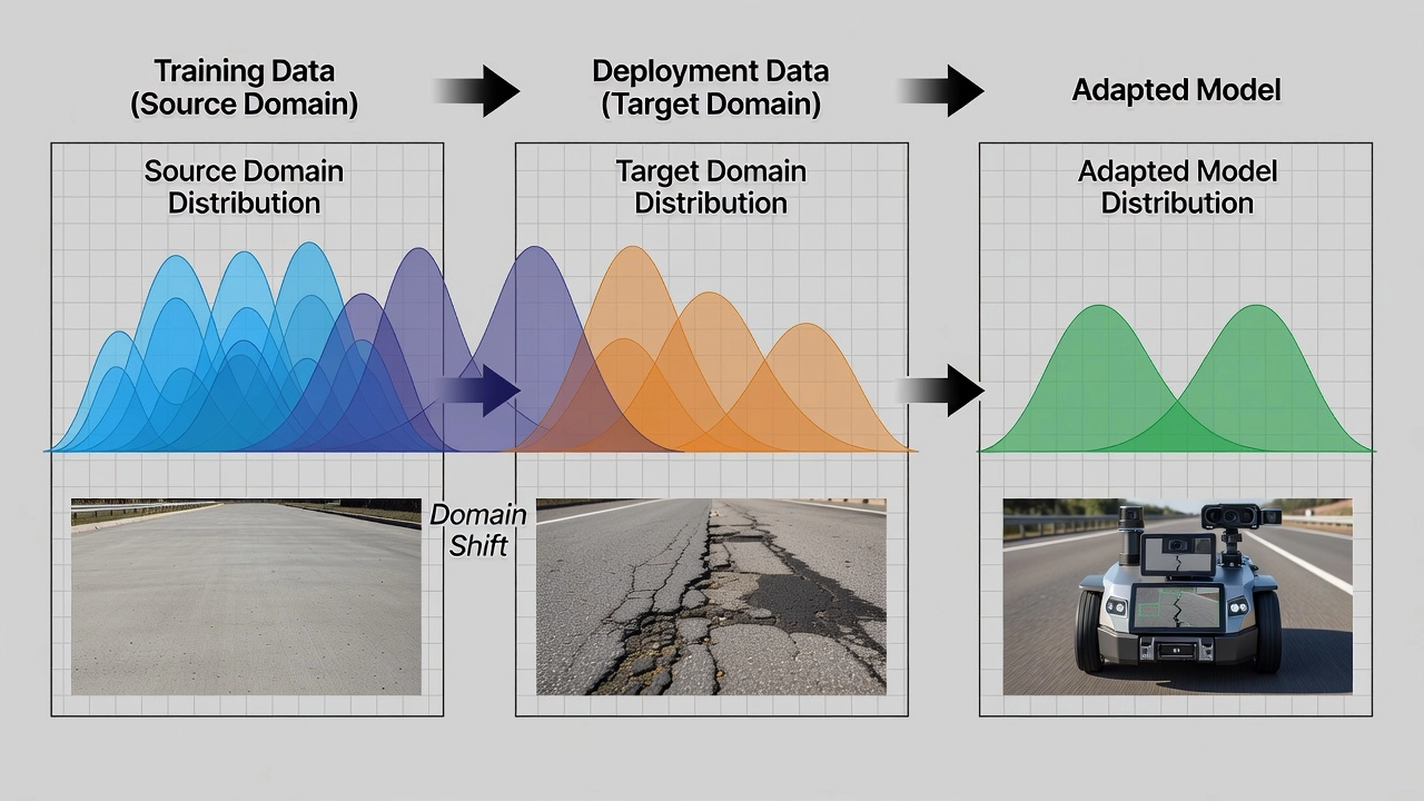
Domain shift (also called distribution shift or dataset shift) is the phenomenon where the data distribution differs between training and deployment environments. When domain shift occurs, model performance degrades because the learned mapping from inputs to outputs no longer matches the target conditions. Domain shift manifests in three principal forms. Covariate shift occurs when the distribution of input features changes while the conditional distribution of labels given inputs remains the same: formally, (P_S(X) \neq P_T(X)) but (P_S(Y|X) = P_T(Y|X)). This is the most common form in computer vision — the visual appearance of a crack on asphalt differs from a crack on concrete, but the mapping from visual features to the label “cracked” remains consistent. Label shift (or prior shift) occurs when the distribution of class labels changes: (P_S(Y) \neq P_T(Y)) but (P_S(X|Y) = P_T(X|Y)). This happens when crack density differs between training and deployment sites. Concept shift occurs when the relationship between inputs and outputs changes: (P_S(Y|X) \neq P_T(Y|X)) — for example, when a visual pattern that indicates a sealed crack on roads indicates a structural defect on runways.
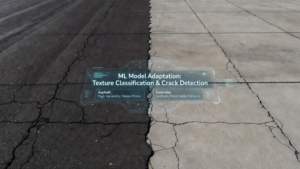
For computer vision in infrastructure inspection, domain shift arises from multiple compounding factors. Visual appearance differences include pavement texture (rough asphalt vs smooth concrete), color profiles (dark gray asphalt vs light gray concrete), and aging patterns (oxidized surface vs freshly paved). Capture conditions such as lighting (direct sunlight at 60° angle vs overcast diffuse light), camera resolution and sensor spectral sensitivity, and image capture angle (nadir from UAV vs oblique from vehicle) all contribute significant distributional shifts. Environmental factors including wet vs dry surfaces, shadow occlusion from structures, and seasonal debris (leaves, snow, standing water) further compound the problem. Surface material differences between asphalt and concrete, or between aged and freshly paved surfaces, represent one of the most challenging domain shifts for pavement inspection models.
Research has documented the severity of domain shift in pavement crack detection quantitatively. The DDACRN framework reported that without domain adaptation, crack detection mean Intersection over Union (mIoU) drops from 0.72 on source test data to 0.31 on cross-dataset target data — a 57% performance reduction. DACrack demonstrated that domain-shift mitigation via multi-level feature alignment recovers approximately 20 percentage points in F1-score on cross-dataset transfers. These empirical results underscore why domain adaptation is not merely an academic refinement but an operational necessity for any inspection system deployed across multiple airports, roads, or bridge networks.
Infrastructure inspection images are subject to multiple interacting sources of domain shift that compound one another. Understanding each source is essential for designing effective adaptation strategies.
Surface material shift is the most prominent domain shift in infrastructure inspection. Asphalt and concrete pavements have fundamentally different visual characteristics. Asphalt is dark gray to black in color, has a coarse and irregular surface texture, and cracks typically appear as bright linear features against the dark background. Concrete is light gray to white, has a smoother and more uniform surface, and cracks appear as dark lines. These differences mean that a convolutional neural network trained on one surface type learns filters and feature representations specific to that surface’s visual statistics. When applied to the other surface type, these filters produce feature activations that the classifier layers cannot interpret correctly. Data from DDACRN shows that cross-surface mIoU drops from 0.72 to 0.31 without adaptation when transferring from asphalt-trained to concrete-tested models.
Crack morphology variation introduces another layer of domain shift. Different pavement distress types have distinct visual signatures. Longitudinal cracks run parallel to the pavement centerline and appear as long, continuous linear features. Transverse cracks run perpendicular to the centerline. Alligator (fatigue) cracks form interconnected networks of small polygons resembling alligator skin. Hairline cracks measure less than 1 mm in width and may be barely visible, while wide cracks exceed 5 mm and are easily identifiable. Sealed cracks filled with sealant material have different visual appearance than unsealed cracks. A model trained predominantly on longitudinal cracks may fail to detect alligator cracking in a target domain where that distress type is more prevalent.
Lighting condition shift significantly affects model performance. Models trained on well-lit daytime images captured under direct sunlight fail on low-light or dusk images, images with harsh shadows cast by structures or trees, and images captured under overcast conditions where diffuse lighting reduces contrast. The angle of incident light relative to the surface normal changes the appearance of crack edges — low-angle sunlight emphasizes surface texture by casting shadows within cracks, while high-angle overhead sun minimizes crack visibility. Shadow occlusion from bridge superstructures, airport terminal buildings, or nearby structures produces localized dark regions where crack features are suppressed. Studies have documented 5–12% accuracy drops for crack detection models when lighting conditions shift from the training distribution.
Camera and sensor shift arises from differences in imaging hardware. Different cameras produce different image resolutions (12 MP smartphone vs 50 MP DSLR vs specialized industrial camera), different color profiles and sensor spectral sensitivity curves, different lens distortion characteristics, and different noise patterns. For UAV-based inspection, flight altitude determines Ground Sampling Distance (GSD) — the physical distance on the ground represented by each pixel. A UAV flying at 30 m produces approximately 0.5–1 cm/pixel GSD, while one at 100 m produces 2–5 cm/pixel. Differences in GSD mean that the same crack is represented by different numbers of pixels and different spatial frequency content in source vs target domains. Fine-tuning with Batch Normalization (BN) statistics recomputation is often sufficient for moderate camera shifts, while severe shifts require adversarial domain alignment at multiple feature levels.
Seasonal and environmental shift introduces temporal domain variation. A model trained on summer images must perform in winter conditions where surfaces may be wet, snow-covered, or partially obscured by fallen leaves. Pavement surfaces undergo aging and oxidation over time, changing their color and texture. The FAA and ICAO Global Reporting Format (GRF) explicitly recognizes environmental condition as a variable that affects runway surface assessment: dry, wet, slippery wet, and contaminated surfaces each represent distinct visual domains requiring different inspection interpretation.
| Domain Shift Source | Typical Performance Impact | Primary Mitigation Strategy |
|---|---|---|
| Surface material (asphalt vs concrete) | 30–45% mIoU drop | Adversarial DA + multi-level feature alignment |
| Lighting condition (sunny vs overcast) | 5–12% accuracy drop | BN adaptation + photometric augmentation |
| Camera resolution / sensor | 3–8% accuracy drop | Fine-tuning + BN statistics recomputation |
| Seasonal / environmental | 8–20% accuracy drop | Generative domain translation (CycleGAN) |
| Geographical / regional | 10–25% accuracy drop | Multi-source UDA + progressive domain bridging |
Fine-tuning is the simplest and most widely used domain adaptation strategy. It involves taking a neural network pre-trained on the source domain and continuing the training process on target domain data, updating the model’s weights to align its representations with the target distribution. Fine-tuning bridges the gap between transfer learning (where the task changes) and domain adaptation (where the task remains the same but the data distribution changes).
The theoretical foundation of fine-tuning rests on the observation that neural networks learn hierarchical feature representations. Early layers capture low-level features such as edges, textures, and color blobs that are largely domain-agnostic. Middle layers combine these into mid-level patterns such as crack edges, surface grain, and joint boundaries. Late layers learn task-specific features optimized for the classification or segmentation objective. When the domain shifts, the low-level statistics (color distributions, texture frequencies, contrast characteristics) change, and the later layers that are finely tuned to source-domain feature distributions lose their alignment.
Full fine-tuning updates all model parameters on target data. This is appropriate when abundant labeled target data is available (hundreds to thousands of images) and computational resources permit full gradient updates. The learning rate is typically reduced by a factor of 10 relative to initial pre-training to prevent catastrophic forgetting — the phenomenon where the model overwrites useful source-domain knowledge. Early stopping based on target validation loss is essential to balance source knowledge retention with target adaptation.
Last-layer (classifier) tuning freezes all feature extraction layers and trains only the final classification or segmentation head. This approach assumes that the feature extractor learned on the source domain produces representations that are sufficiently general, and only the mapping from features to labels needs adjustment. Last-layer tuning is effective when very limited target data is available (tens of images) and the domain shift is primarily in the label space rather than the feature space. It requires minimal computation and is resistant to catastrophic forgetting.
Progressive unfreezing provides a middle ground. The training process starts with all layers frozen except the final classifier, which is trained for several epochs. Then, the topmost feature extraction layers are unfrozen and trained together with the classifier. This process continues, gradually unfreezing layers from top to bottom, until all layers are fine-tuning or a performance plateau is reached. Progressive unfreezing is appropriate for moderate amounts of target data (hundreds of images) and domain shifts that affect multiple levels of feature hierarchy.
Adapter modules introduce small bottleneck layers with significantly fewer parameters than the full network. These adapters are inserted between the layers of a frozen pre-trained backbone and are the only parameters updated during fine-tuning. Adapter-based fine-tuning is highly parameter-efficient — typically 1–5% of the total parameter count — and enables rapid switching between multiple target domains by storing and loading different adapter weights. For infrastructure inspection networks with millions of parameters, adapter modules enable deployment across dozens of airports without storing separate full-weight copies for each.
Batch Normalization (BN) adaptation is a remarkably lightweight yet effective technique. BN layers compute running mean and variance statistics during training to normalize intermediate feature maps. When the domain shifts, these statistics no longer accurately represent the target distribution. BN adaptation simply recomputes the BN statistics by passing target domain data through the network with frozen weights, updating the running mean and variance without any gradient updates. This alone can significantly reduce domain shift when the primary difference is in low-level image statistics such as brightness, contrast, and color distribution. Studies on crack detection show BN adaptation recovers 3–8% of accuracy drops caused by moderate lighting and camera shifts, requiring only a single forward pass of unlabeled target data.
| Fine-Tuning Strategy | Target Data Required | Parameters Updated | Catastrophic Forgetting Risk | Best Use Case |
|---|---|---|---|---|
| BN statistics recomputation | None (unlabeled) | 0 (BN stats only) | None | Lighting / camera shifts |
| Last-layer tuning | 10–50 labeled | < 1% | Very low | Feature distribution preserved |
| Adapter modules | 50–200 labeled | 1–5% | Low | Multi-domain deployment |
| Progressive unfreezing | 100–500 labeled | Gradual, 10–100% | Moderate | Moderate domain shift |
| Full fine-tuning | 500+ labeled | 100% | High | Abundant target data; large shift |
Supervised domain adaptation (SDA) operates under the assumption that a small amount of labeled data is available in the target domain alongside abundant labeled source data. This is the most straightforward setting: the model has direct access to ground-truth information about the target domain, enabling explicit optimization for target performance.
The standard SDA approach has two components. First, the model is pre-trained on the source domain with its abundant labels — this establishes general knowledge about the inspection task, learning to recognize crack edges, joint boundaries, surface textures, and defect geometries. Second, the model is fine-tuned on the labeled target data using a substantially reduced learning rate. During fine-tuning, the loss function typically combines source and target losses to prevent the model from forgetting useful source-domain knowledge. The combined loss is expressed as:
(\mathcal{L}_{\text{SDA}} = \mathcal{L}_S(\theta) + \lambda \mathcal{L}_T(\theta))
where (\mathcal{L}_S) is the source loss computed on source data, (\mathcal{L}_T) is the target loss computed on labeled target data, and (\lambda) controls the relative contribution of each domain. During training, source and target batches are alternately or jointly fed through the network.
Key techniques for supervised domain adaptation include weighted loss functions that give higher importance to target domain samples during fine-tuning, joint training where source and target labeled data are mixed in each training batch, and domain adversarial training where a domain classifier is added even in the supervised setting to encourage the feature extractor to learn domain-invariant representations. Curriculum learning strategies start with source-dominated training and gradually shift the balance toward target data as training progresses.
Parameter transfer — where the source-trained model’s weights serve as initialization — is the dominant strategy in SDA. The success of this approach depends on the degree of relatedness between source and target domains. When the domains are closely related (e.g., different sections of the same airport pavement), very few labeled target examples are sufficient — as few as 20–50 images can recover most of the performance lost to domain shift. When domains are more distant (e.g., road to runway), 200–500 labeled target examples are typically required for robust adaptation.
Label-efficient SDA techniques aim to minimize the number of target labels needed. Active learning identifies the most informative target samples for labeling: the model is trained on source data, applied to unlabeled target data, and the samples where it is most uncertain are selected for human labeling. This approach can reduce labeling requirements by 50–70% compared to random sampling. Self-training (or pseudo-labeling) applies the source-trained model to unlabeled target data, generates provisional labels for high-confidence predictions, and retrains the model using these pseudo-labels as additional supervision. Self-training is particularly effective when combined with confidence thresholding and data augmentation.
When to use SDA: when obtaining a small labeled set from each target deployment site is feasible. For airport runway inspection, this means a trained inspector can label 50–200 images per airport — a one-time cost of 1–4 hours per site. This is far more economical than the alternative of collecting and labeling thousands of images per airport, which would require multiple days per site. The FAA AC 150/5380-6C recommends regular PCI surveys that already involve inspectors examining pavement surfaces — these same inspectors can provide the few hundred labeled images needed for SDA as part of their standard inspection workflow.
Unsupervised domain adaptation (UDA) is the most challenging and actively researched domain adaptation setting. It assumes that labeled data exists only in the source domain, while the target domain is completely unlabeled. UDA is the dominant scenario for infrastructure inspection because labeling target domain data is expensive, time-consuming, or impractical across many deployment sites. A model trained on one airport’s pavement images must adapt to a different airport’s surfaces, lighting, and defect patterns without requiring every airport to produce a labeled dataset.
UDA methods fall into three major categories: adversarial methods, discrepancy-based methods, and reconstruction-based methods. All share the core objective of aligning source and target feature distributions so that a classifier trained on source features generalizes to target features.
Adversarial domain adaptation draws inspiration from Generative Adversarial Networks (GANs). The core idea is to train a domain discriminator (a binary classifier that predicts whether a feature representation came from the source or target domain) alongside the feature extractor in a minimax game. The feature extractor tries to produce features that are indistinguishable between source and target, while the discriminator tries to correctly identify each feature’s origin.
The canonical architecture is the Domain-Adversarial Neural Network (DANN), introduced by Yaroslav Ganin and Victor Lempitsky in 2015. DANN consists of three components: a feature extractor (G_f) that maps inputs to a feature space (f = G_f(x; \theta_f)); a label predictor (G_y) that maps features to task labels (\hat{y} = G_y(f; \theta_y)); and a domain classifier (G_d) that maps features to domain labels (\hat{d} = G_d(f; \theta_d)). The critical innovation is the Gradient Reversal Layer (GRL) placed between the feature extractor and the domain classifier. During forward propagation, the GRL acts as an identity transformation. During backpropagation, it multiplies the gradient by (-\lambda), where (\lambda) is a hyperparameter controlling the adaptation strength. This reversal causes the feature extractor to learn features that maximize domain classification loss — effectively learning to fool the domain classifier.
The DANN loss function combines task loss on source labels minus the domain classification loss on both source and target features:
(\mathcal{L}(\theta_f, \theta_y, \theta_d) = \frac{1}{n_S}\sum_{x_i \in D_S} \mathcal{L}y(G_y(G_f(x_i)), y_i) - \frac{\lambda}{n_S + n_T}\sum{x_i \in D_S \cup D_T} \mathcal{L}_d(G_d(G_f(x_i)), d_i))
As training progresses, the feature extractor learns representations that are both discriminative for the task (because the label predictor is trained on source labels) and domain-invariant (because the domain classifier cannot distinguish domain origin). The GRL scheduling typically starts with (\lambda = 0) and gradually increases to a maximum value over the first few epochs, allowing the network to stabilize its task performance before the domain confusion pressure is applied.
Recent advances in adversarial domain adaptation include Contrastive Adversarial Training (CAT), which leverages labeled source samples to reinforce feature separation while maintaining domain alignment; Collaborative and Adversarial Networks (CAN), which perform multi-level domain alignment at different feature hierarchy levels; and Adversarial Style Discrepancy Minimization, which uses style transfer as an adversarial objective. For pavement crack detection, adversarial methods have demonstrated the strongest cross-dataset generalization, recovering 15–25 percentage points of the performance lost to domain shift.
Discrepancy-based methods take a different approach: instead of adversarial training, they explicitly minimize a statistical distance measure between source and target feature distributions. The advantage is training stability — no adversarial dynamics that require careful hyperparameter tuning — at the cost of potentially weaker alignment.
Maximum Mean Discrepancy (MMD) is the most widely used discrepancy measure for domain adaptation. MMD is a kernel-based statistical test that measures the distance between two distributions in a Reproducing Kernel Hilbert Space (RKHS). Given source features (\mathbf{f}^S) and target features (\mathbf{f}^T), the squared MMD is:
(MMD^2(\mathbf{f}^S, \mathbf{f}^T) = \left|\frac{1}{n_S}\sum_{i=1}^{n_S}\phi(f_i^S) - \frac{1}{n_T}\sum_{j=1}^{n_T}\phi(f_j^T)\right|_{\mathcal{H}}^2)
where (\phi) is the feature map into the RKHS. In practice, the MMD is computed using a kernel function (k(x,y) = \langle \phi(x), \phi(y) \rangle) — typically the Gaussian RBF kernel, often with multiple bandwidths to capture different levels of distribution similarity.
Deep Adaptation Networks (DAN), introduced by Long et al. in 2015, add MMD loss to multiple task-specific layers of a deep CNN. The total loss becomes (\mathcal{L} = \mathcal{L}S + \lambda \sum{l \in L} MMD^2(\mathbf{f}_l^S, \mathbf{f}_l^T)), where (L) is the set of layers at which domain alignment is applied. DAN demonstrated that aligning higher-level feature representations (rather than just the final layer) significantly improves adaptation quality.
CORrelation ALignment (CORAL), introduced by Sun and Saenko in 2016, takes a simpler approach by minimizing the difference between source and target feature covariance matrices:
(\mathcal{L}_{CORAL} = \frac{1}{4d^2}|C_S - C_T|_F^2)
where (C_S) and (C_T) are the feature covariance matrices of source and target respectively, (d) is the feature dimension, and (|\cdot|_F) is the Frobenius norm. Deep CORAL extends this to deep networks by adding the CORAL loss to the network’s loss function. CORAL is computationally efficient and performs well when domain shift is primarily in feature variance rather than mean.
Joint Adaptation Networks (JAN) extend DAN by aligning the joint distributions of multiple layers rather than treating each layer independently. JAN uses Joint MMD (JMMD), defined on the tensor product of activations from multiple layers. This captures inter-layer dependencies that individual MMD losses miss.
Recent advances for infrastructure inspection include the framework by Wang et al. (2025) for corrosion segmentation, which combines three complementary discrepancy modules: Geometric Structure Preservation (GSP) that retains local topological relationships across domains using graph-based regularization; SVD-based Local Discrepancy (SLD) that uses singular value decomposition to align local feature subspaces at a fine-grained level; and Global Consistency Alignment (GCA) that uses MMD to reconcile global distributional shifts. This combined approach, supported by the lightweight EffSegNet segmentation backbone, achieved strong cross-domain generalization from laboratory corrosion imagery to field conditions on locks, dams, and transportation infrastructure.
| Method | Category | Alignment Mechanism | Training Stability | Infrastructure Performance |
|---|---|---|---|---|
| DANN | Adversarial | Gradient reversal + domain classifier | Moderate (requires tuning (\lambda)) | Strong (recovers 15–25 ppt mIoU) |
| DAN | Discrepancy | MMD on multiple layer outputs | High | Good (recovers 10–20 ppt mIoU) |
| Deep CORAL | Discrepancy | Covariance alignment (2nd-order stats) | High | Moderate (recovers 8–15 ppt mIoU) |
| JAN | Discrepancy | Joint MMD on layer pairs | High | Good (recovers 12–18 ppt mIoU) |
| CycleGAN+Det | Generative | Image-to-image translation + task model | Low (GAN training difficulty) | Strong when image translation succeeds |
| CAT | Adversarial | Contrastive + adversarial | Moderate | Strong (state-of-the-art on several benchmarks) |
Domain-invariant features are feature representations produced by a neural network that have the same statistical distribution regardless of which domain the input originates from. If (f(x)) is the feature representation extracted by the network, domain invariance means (P(f(X_S)) \approx P(f(X_T))). The goal is to learn a mapping (f) such that the distance (d(P(f(X_S)), P(f(X_T)))) is minimized while preserving task-specific discriminative power.
The four principal approaches to learning domain-invariant features each handle the invariance-discriminability trade-off differently. Adversarial learning (DANN, GAN-based) pushes the feature extractor to produce features that a domain discriminator cannot distinguish. This is the most aggressive invariance mechanism but risks removing task-relevant information if crack texture correlates with surface type. Statistical moment matching (MMD, CORAL) aligns distribution moments — first-order (mean) and second-order (covariance) — between source and target features. This preserves more task-relevant information than full adversarial alignment but may not capture higher-order distribution differences. Optimal transport (OT-based methods) finds a minimal-cost mapping between source and target distributions, providing a geometric interpretation of domain alignment. Style transfer and generative methods (CycleGAN, StarGAN) transform images from one domain to visually resemble another before passing them through the task network. This operates at the pixel level rather than the feature level and has the advantage of producing interpretable transformed images.
The invariance-discriminability trade-off is a fundamental tension in domain-invariant feature learning. Maximizing domain invariance may remove task-relevant information that correlates with the domain. For example, if crack edges on asphalt have higher contrast than on concrete, a feature detector that relies on edge contrast strength will be sensitive to both crack presence and pavement type. Forcing complete invariance to pavement type may suppress the edge contrast features needed for crack detection. Advanced methods address this through multi-level alignment — aligning only higher-level semantic features while retaining low-level texture cues — and conditional alignment that aligns distributions conditioned on the task label, preserving class-discriminative information.
Attention-based domain invariance leverages attention mechanisms to focus on domain-agnostic semantic regions. A crack detection model with a spatial attention module learns to attend to crack structures regardless of background pavement texture. The attention maps themselves become more domain-invariant than the raw feature maps because they highlight task-relevant spatial locations while suppressing domain-specific background. Cross-attention between source and target features further strengthens this by explicitly matching attended regions across domains.
Self-supervised domain adaptation methods use pretext tasks such as rotation prediction, jigsaw puzzle solving, or contrastive instance discrimination to learn features that are robust to domain variation without requiring any domain labels. By solving these auxiliary tasks, the model learns to capture structural and geometric properties of the input that are shared across domains. The self-supervised pre-trained features often exhibit stronger domain invariance than purely supervised features because the pretext tasks do not depend on domain-specific label distributions.
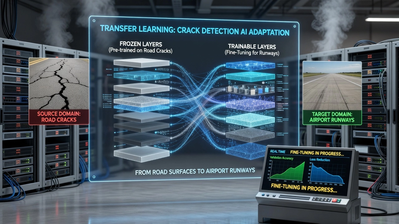
The transition from road pavement inspection to airport runway inspection represents one of the most challenging domain adaptation problems in infrastructure asset management. Roads and runways are fundamentally different engineered structures designed for different loads, speeds, and safety requirements, producing dramatically different visual appearances and defect characteristics.
| Factor | Road Pavement | Airport Runway Pavement |
|---|---|---|
| Design standard | Varies by jurisdiction | ICAO Annex 14 / FAA standards |
| Load per axle | ~10 tons (vehicles) | 50–400 tons (aircraft) |
| Primary surface material | Asphalt (HMA) | High-strength PCC concrete (common) or heavy-duty asphalt |
| Markings | Yellow/white lane markings (multiple colors) | White markings only; complex patterns (threshold, touchdown zone, aiming point, centerline) |
| Primary defect types | Cracks, potholes, rutting, bleeding | Cracks, FOD, rubber deposits, raveling, friction degradation, jet blast erosion, fuel spill damage |
| Inspection access | Public roads; easy unrestricted access | Restricted airside; requires airfield pass, vehicle escort, radio communication |
| Dominant capture method | Ground vehicles, smartphones, manual | UAV at 30–100m altitude, specialized inspection vehicles |
| Surface contaminants | Water, snow, debris, oil | Water, rubber (critical — touchdown zones), de-icing fluids, jet fuel, hydraulic fluid |
| Safety-critical friction parameter | Skid resistance for braking | Braking action coefficient for landing aircraft (ICAO GRF categories) |
| Regulatory framework | FHWA, state DOT standards | ICAO Annex 14, Doc 9137, FAA ACs |
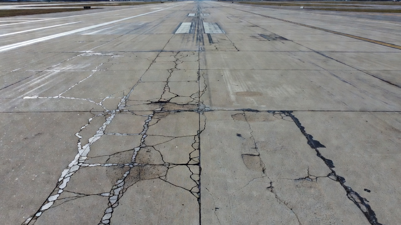
Rubber deposit interference is the single most challenging adaptation issue. Aircraft tires deposit rubber on runways during landing — particularly in the touchdown zone — accumulating as dark, continuous patches on the pavement surface. These rubber deposits can visually mimic or obscure cracks. A road-trained crack detection model, which has never encountered tire rubber deposits, may either fail to detect cracks beneath rubber patches or falsely classify rubber patch edges as cracks. Road-to-runway adaptation must therefore incorporate rubber deposit modeling, either through synthetic augmentation of training data or through domain adaptation methods that learn to distinguish rubber from cracks.
Scale and resolution differences are another significant adaptation barrier. Road inspection images are typically captured from ground level at distances of 1–5 meters, yielding very high resolution where individual crack edges span tens of pixels. Runway inspection using UAVs at 30–100m altitude produces images with coarser resolution — a crack that spans 50 pixels in a road image may span only 5–10 pixels in a runway image captured from altitude. The feature extractor’s receptive fields and scale-dependent filters must adapt to this difference in spatial frequency content. Multi-scale feature pyramids and scale-invariant training are essential adaptation components.
Defect definition mismatch requires careful mapping between road and runway distress taxonomies. The FHWA LTPP Distress Identification Manual defines road pavement defects in categories that partially overlap with airport pavement defects defined by ASTM D5340 and ICAO Doc 9137 Part 9. Some defect types are unique to airfields: rubber deposits, jet blast erosion, fuel spill damage, and friction degradation have no road equivalents. Road-trained models therefore need new output classes added during adaptation, or a hierarchical classification approach that first detects generic defects and then classifies them into domain-specific categories.
Regulatory compliance imposes an additional layer of adaptation requirement. Road inspection models produce outputs that inform maintenance prioritization by DOT agencies. Runway inspection models must produce outputs that map to ICAO- and FAA-mandated reporting formats: the Global Reporting Format (GRF) condition categories, the Pavement Condition Index (PCI) per ASTM D5340, and Pavement Classification Number (PCN) ratings. The adaptation process must therefore also adapt the model’s output representation to align with regulatory reporting standards.
Progressive domain bridging — training on intermediate datasets that gradually span the gap from road to runway — has proven effective. A typical bridging pipeline uses three stages: first, train on road datasets (CQU-BPDD, RDD2020, Crack500); second, adapt to general pavement datasets that include both asphalt and concrete surfaces; third, adapt to runway-specific datasets with rubber deposits and airfield markings. Each stage reduces the distribution gap that the next stage must bridge, enabling more stable and effective adaptation than direct road-to-runway transfer.
Climate conditions introduce domain variation that is temporal (changing over time at a single location) and geographical (varying across locations simultaneously). A model deployed across multiple airports must handle both dimensions.
Wet vs dry surface adaptation is critical because runway surface condition categories under the ICAO Global Reporting Format explicitly distinguish dry, wet, slippery wet, and contaminated surfaces. Wet surfaces alter crack visibility in several ways. Water filling cracks reduces the contrast between the crack and the surrounding pavement — dry cracks appear as high-contrast dark or bright linear features, but water-filled cracks appear as low-contrast features that may be nearly invisible to a model trained on dry surfaces. Water sheeting on the pavement surface creates specular reflections that introduce bright regions and false edges, confusing crack detectors. Wet pavement also appears darker overall, shifting the image histogram and altering the statistics of every layer in the network.
Cold climate adaptation addresses freeze-thaw effects that change pavement appearance. Frozen surfaces have different reflectance properties than unfrozen surfaces. Ice patches on pavement appear as smooth, high-reflectivity regions that share visual characteristics with pavement surface defects. Snow cover partially or completely obscures surface defects. The transition between freezing and thawing cycles produces unique distress patterns — D-cracking, freeze-thaw spalling, and frost heave — that models trained on warm-climate data may not recognize.
Data augmentation for climate adaptation synthetically generates target-domain variations from source-domain images. Adding simulated rain streaks, wet surface reflectance models, snow cover masks, and shadow overlays can expand the source domain’s coverage to include climate conditions not present in the original training data. RandAugment policies with specific photometric transforms targeting brightness, contrast, and color temperature shifts are particularly effective for climate adaptation. Studies show that augmentation-only approaches recover 50–70% of the performance lost to lighting and weather domain shifts, making them a cost-effective complement to more complex adversarial or discrepancy-based methods.
CycleGAN-based domain translation provides an alternative by learning to translate images between climate conditions. A CycleGAN trained on paired or unpaired images from dry and wet runways learns to map from the dry domain to the wet domain while preserving crack locations and geometries. Crack detection models trained on this augmented data learn features that are invariant to the presence or absence of water on the surface. The disadvantage is the training complexity of GANs and the risk of hallucinating or removing crack features during translation.
Infrastructure inspection systems use a variety of imaging platforms, each with different optical characteristics that introduce domain shift. Adaptation across camera types is essential for any system deployed across multiple airports, where existing imagery may come from different sources.
Resolution and Ground Sampling Distance (GSD) vary widely. Ground-level inspection with a 50 MP DSLR produces GSDs of 0.1–0.5 mm/pixel. UAV inspection at 30 m altitude produces 0.5–1 cm/pixel. UAV inspection at 100 m altitude produces 2–5 cm/pixel. Satellite imagery may have 30–50 cm/pixel resolution. A crack that is 3 mm wide spans 6–30 pixels at ground level, 0.3–0.6 pixels at 30 m UAV altitude, and is sub-pixel at 100 m. Models trained on high-resolution ground images cannot directly detect features at coarser resolutions. Multi-resolution training — training on images at multiple resolution scales — is the primary strategy. The feature extractor learns scale-invariant representations through pyramid pooling, dilated convolutions, or resolution-adaptive normalization.
Sensor spectral sensitivity differences between cameras affect color representation. Different CMOS and CCD sensors have different quantum efficiency curves across the visible spectrum, meaning the same surface appears with slightly different RGB values from different cameras. Color calibration using a color checker chart during data collection reduces this shift but is rarely practical for large-scale inspection programs. Histogram matching and color transfer between source and target images are preprocessing alternatives. More sophisticated approaches include sensor-invariant feature learning that explicitly removes sensor-specific color information from feature representations through color jitter augmentation during training.
Lens distortion varies across camera and lens combinations. Wide-angle lenses used for efficient runway coverage introduce barrel distortion that changes crack geometry — straight cracks may appear curved near image edges. For detection tasks, this distortion affects the spatial relationship between image features. Distortion correction as a preprocessing step normalizes all images to a common rectified geometry before feeding them to the model. Alternatively, training on images with synthetic distortion augmentation makes the model robust to varying distortion levels.
Rolling shutter effects from UAV platforms introduce geometric distortion during flight — particularly at high speed or in windy conditions. The sequential exposure of rows in a rolling shutter CMOS sensor means that camera motion during exposure produces skewed or warped crack geometry. This temporal distortion is absent in global shutter cameras and in ground-level static capture. Adaptation requires either preprocessing to correct rolling shutter artifacts or training on data that includes synthetic rolling shutter degradation.
| Camera Variation | Adaptation Strategy | Implementation Complexity | Typical Recovery |
|---|---|---|---|
| Resolution / GSD | Multi-resolution training + pyramid pooling | Moderate | 5–10% accuracy recovery |
| Sensor color response | Color jitter augmentation + histogram matching | Low | 3–7% accuracy recovery |
| Lens distortion | Distortion correction preprocessing | Low | 2–5% accuracy recovery |
| Rolling shutter | Synthetic rolling shutter augmentation | Moderate | 3–6% accuracy recovery |
| Compression artifacts | JPEG compression augmentation | Low | 1–3% accuracy recovery |
TarmacView implements domain adaptation as a core capability of its inspection model training infrastructure. The platform recognizes that no single airport deployment will perfectly match the training conditions of another, and that per-site model retraining is economically infeasible. The domain adaptation pipeline provides multiple adaptation pathways that can be selected based on the amount and type of target data available.
The TarmacView fine-tuning pipeline supports three tiers of domain adaptation. Full fine-tuning is available when customers provide 500+ labeled images from the target airport. The process starts from a pre-trained base model (trained on a diverse multi-airport, multi-surface dataset), reduces the learning rate by 10x, and trains for 50–100 epochs with early stopping. Progressive unfreezing is the default strategy, unfreezing the classifier head first, then the top two encoder blocks, then the full network if target performance has not plateaued. Adapter-based fine-tuning is the recommended approach for 50–200 labeled target images. Lightweight adapter modules are inserted into the pre-trained backbone and trained with the target data while the backbone remains frozen. Adapter modules for each airport are stored independently, enabling rapid switching between airport-specific models without loading full weight copies. Unsupervised adaptation via BN statistics recomputation and feature alignment is used when no labeled target data is available. The model processes unlabeled target images in a forward pass, recomputes BN running statistics, and optionally applies feature alignment losses (CORAL or MMD) to minimize distribution shift without requiring any ground-truth labels.
Domain-adaptation-fine-tuned variants are generated for each deployment scenario. These variants combine the pre-trained base model with target-specific adjustments including BN statistics from the target domain, adapter module weights if adapter-based tuning was performed, and target-specific data augmentation configurations tuned to the imaging conditions at the target airport. The resulting model retains the broad knowledge of the base model while incorporating targeted adjustments for the specific deployment environment.
The domain gap assessment module is a diagnostic tool that evaluates the magnitude and nature of domain shift before adaptation. The module collects a sample of unlabeled target images, extracts features using the source model, and computes distribution distance metrics (MMD, CORAL distance, entropy of predictions) between source validation data and target data. The results guide the selection of adaptation strategy: low MMD suggests BN adaptation is sufficient, moderate MMD suggests adapter-based fine-tuning, high MMD suggests full fine-tuning or unsupervised adversarial alignment. The assessment also identifies which layers of the network are most affected by domain shift, enabling targeted adaptation rather than blanket application of domain alignment to all layers.
Monitoring domain drift over time is an operational capability. As airport pavement ages, undergoes maintenance, or experiences seasonal changes, the visual domain may drift away from the conditions at the time of model deployment. TarmacView’s monitoring pipeline periodically collects unlabeled images during routine inspection flights, recomputes distribution distance metrics, and triggers re-adaptation if the drift exceeds a configurable threshold. This continuous adaptation cycle ensures that deployed models maintain accuracy over the operational lifetime of the inspection program, adapting to pavement aging, new surface treatments, camera replacements, and seasonal variation without requiring manual intervention.
Performance validation compares adapted model performance against non-adapted baselines using held-out target test data. Standard metrics include F1-score for crack detection, mIoU for defect segmentation, and per-class accuracy for defect classification. The validation pipeline also reports domain-specific metrics such as adaptation gain — the improvement in target performance relative to the non-adapted baseline — and source retention — the performance maintained on source domain data after adaptation — to quantify the invariance-discriminability trade-off for each deployment.
The economic impact of domain adaptation is substantial. Without domain adaptation, each airport deployment would require collecting and labeling 2,000–5,000 images — a process costing $5,000–15,000 per airport in labeling alone, plus data collection costs. With unsupervised domain adaptation and optional adapter-based fine-tuning, labeling costs are eliminated or reduced to 50–200 images ($125–500 per airport). For an operator managing 20 airports, domain adaptation reduces inspection AI deployment costs from $100,000–300,000 to $2,500–10,000, while maintaining crack detection accuracy within 2–5% of the fully supervised upper bound.
Understanding domain adaptation requires familiarity with several core mathematical formulations. The Empirical Risk Minimization (ERM) framework provides the starting point. Given a source domain with labeled samples ({(x_i^S, y_i^S)}_{i=1}^{n_S}), a standard model minimizes the empirical risk:
(\hat{R}S(\theta) = \frac{1}{n_S}\sum{i=1}^{n_S} \ell(f_\theta(x_i^S), y_i^S))
where (\ell) is the task-specific loss function (cross-entropy for classification, Dice loss for segmentation). Domain adaptation aims to minimize the target risk:
(R_T(\theta) = \mathbb{E}{(x, y) \sim P_T}[\ell(f\theta(x), y)])
The challenge is that (R_T) cannot be directly minimized when target labels are unavailable. Domain adaptation methods bound the target risk by the sum of the source risk and a divergence measure between source and target distributions.
The H-divergence provides a theoretical bound for domain adaptation (Ben-David et al., 2010). For a hypothesis class (\mathcal{H}), the H-divergence between source and target distributions is:
(d_{\mathcal{H}}(D_S, D_T) = 2 \sup_{h \in \mathcal{H}} \left| \Pr_{x \sim D_S}[h(x) = 1] - \Pr_{x \sim D_T}[h(x) = 1] \right|)
In practice, the H-divergence is estimated by training a classifier to discriminate between source and target domain samples — exactly what the domain classifier in DANN does. The theoretical result guarantees that a model trained on source data will generalize to the target domain if the H-divergence between the domains is small. This provides the formal justification for adversarial domain adaptation.
The MMD in functional form uses a characteristic kernel (k) to embed probability distributions in an RKHS:
(MMD(P_S, P_T) = \sup_{|f|{\mathcal{H}} \leq 1} (\mathbb{E}{x \sim P_S}[f(x)] - \mathbb{E}_{x \sim P_T}[f(x)]))
With the Gaussian kernel (k(x, y) = \exp(-|x - y|^2 / 2\sigma^2)), the squared MMD can be computed directly from sample means:
(MMD^2 = \frac{1}{n_S^2}\sum_{i,j} k(x_i^S, x_j^S) + \frac{1}{n_T^2}\sum_{i,j} k(x_i^T, x_j^T) - \frac{2}{n_S n_T}\sum_{i,j} k(x_i^S, x_j^T))
The CORAL loss aligns second-order statistics:
(\mathcal{L}_{CORAL} = \frac{1}{4d^2}|C_S - C_T|_F^2)
where (C_S = \frac{1}{n_S - 1}(\mathbf{F}_S^\top \mathbf{F}_S - \frac{1}{n_S}(\mathbf{1}^\top \mathbf{F}_S)^\top (\mathbf{1}^\top \mathbf{F}_S))) and (C_T) is defined analogously for target features. The Frobenius norm (|\cdot|_F) is the element-wise sum of squares.
These mathematical foundations translate directly to practical implementation. The domain adaptation loss for a Deep CORAL network is:
(\mathcal{L} = \mathcal{L}{task}(D_S, Y_S) + \lambda{CORAL} \cdot \mathcal{L}_{CORAL}(\mathbf{F}_S, \mathbf{F}_T))
For a DANN network:
(\mathcal{L} = \mathcal{L}{task}(D_S, Y_S) - \lambda{DANN} \cdot \mathcal{L}_{domain}(\mathbf{F}_S, \mathbf{F}_T, \mathbf{D}))
where (\mathbf{D} = {0, 1}) indicates source (0) or target (1) domain, and the negative sign reflects the gradient reversal.
| Method | Objective Function | Key Hyperparameters |
|---|---|---|
| ERM (no adaptation) | (\mathcal{L} = \mathcal{L}_{task}(D_S, Y_S)) | Learning rate, weight decay |
| DANN | (\mathcal{L} = \mathcal{L}{task} - \lambda \mathcal{L}{domain}) | (\lambda) (adaptation strength), GRL schedule |
| DAN | (\mathcal{L} = \mathcal{L}_{task} + \sum_l \lambda_l MMD_l^2) | (\lambda_l) per layer, kernel bandwidth (\sigma) |
| Deep CORAL | (\mathcal{L} = \mathcal{L}_{task} + \lambda |C_S - C_T|_F^2) | (\lambda) (alignment weight) |
| JAN | (\mathcal{L} = \mathcal{L}_{task} + \sum_l \lambda_l JMMD_l) | Layer pairs, kernel bandwidths |
| Fine-tuning | (\mathcal{L} = \mathcal{L}_{task}(D_T, Y_T)) reduced LR | Freeze schedule, LR reduction factor |
Evaluating domain adaptation methods requires standardized cross-dataset benchmarks that measure performance on target domains not seen during training. For infrastructure inspection, several benchmark protocols have been established.
Cross-dataset evaluation is the standard protocol. The model is trained on a source dataset (e.g., CQU-BPDD, which contains bituminous pavement crack images) and evaluated on a target dataset (e.g., RDD2020, which contains road crack images from multiple countries). The performance on the target dataset before adaptation serves as the source-only baseline. Performance after adaptation (with access to unlabeled target data for UDA or limited labeled target data for SDA) is measured against this baseline. The adaptation gain — the difference between adapted and unadapted performance — quantifies the effectiveness of the adaptation method.
Common benchmarks for pavement crack detection include: CQU-BPDD (Bituminous Pavement Crack Dataset) containing 60,088 images of asphalt pavement cracks from China; RDD2020 containing 26,336 images of road cracks from India, Japan, and the Czech Republic; Crack500 containing 500 high-resolution images of pavement cracks from road surfaces; DeepCrack containing 537 images of building wall cracks; and SDNET2018 containing 56,000 images of concrete bridge decks, walls, and pavements. Cross-dataset evaluation across these datasets — particularly from CQU-BPDD to RDD2020, representing a cross-country and cross-climate transfer — is the most stringent benchmark.
Metrics for domain adaptation assessment include target-domain mIoU (mean Intersection over Union for segmentation tasks), target-domain F1-score (for detection tasks), source retention (source domain performance after adaptation, to measure catastrophic forgetting), adaptation gain (percentage point improvement over source-only baseline), and label efficiency (how much target labeled data is needed to achieve a given performance level for supervised methods).
Statistical significance testing is essential because domain adaptation results can be noisy. Multiple runs with different random seeds (typically 5–10) are used to compute mean and standard deviation of performance metrics. The Wilcoxon signed-rank test or paired t-test is used to determine whether performance differences between adaptation methods are statistically significant at conventional thresholds ((p < 0.05)).
For infrastructure inspection, additional deployment-specific metrics are relevant: false positive rate at operational severity thresholds (a crack detector that generates 100 false alarms per runway inspection is operationally useless regardless of its mIoU); inference time per unit area (adaptation should not significantly increase processing time); and memory footprint (adapter-based methods should add minimal storage overhead per additional airport).
The practice of domain adaptation for infrastructure inspection draws on standards and research from multiple disciplines.
Machine learning foundations: Ganin et al., “Domain-Adversarial Training of Neural Networks” (Journal of Machine Learning Research, 2016) — the canonical DANN paper introducing gradient reversal. Long et al., “Learning Transferable Features with Deep Adaptation Networks” (ICML, 2015) — introducing MMD-based multi-layer domain alignment. Sun and Saenko, “Deep CORAL: Correlation Alignment for Deep Domain Adaptation” (ECCV, 2016) — introducing covariance-based alignment. Ben-David et al., “A theory of learning from different domains” (Machine Learning, 2010) — the theoretical framework for domain adaptation generalization bounds.
Infrastructure inspection domain adaptation: Liu et al., “DDACRN: Deep Domain Adaptation-based Crack Detection Network” (IEEE Transactions on Intelligent Transportation Systems, 2023) — the primary reference for crack detection domain adaptation with two-branch weight-shared architecture. “DACrack: Unsupervised Domain Adaptation for Crack Detection” (Automation in Construction, 2023) — multi-level feature alignment for cross-dataset crack detection. Wang, Nguyen, Eick et al., “Efficient Domain Adaptation Network for Corrosion Segmentation in Infrastructure” (Journal of Civil Structural Health Monitoring, 2025) — three-module discrepancy framework for infrastructure corrosion.
ICAO and FAA standards: ICAO Annex 14 — Aerodromes, Volume I (8th Edition, 2018 with amendments) — primary international standard for aerodrome certification, creating the domain shift context across airports. ICAO Doc 9137, Part 9 — Airport Services Manual, Airport Maintenance Practices — pavement maintenance guidance. ICAO Global Reporting Format (GRF) for Runway Surface Conditions (effective November 2021) — defining surface condition domains (dry, wet, contaminated). FAA AC 150/5380-6C — Guidelines and Procedures for Maintenance of Airport Pavements. ASTM D5340 — Standard Test Method for Airport Pavement Condition Index Surveys — the quantitative framework for pavement condition assessment that domain-adapted models must support.
Pavement datasets: CQU-BPDD (Chongqing University, 60,088 asphalt pavement crack images). RDD2020 (8,300+ road images from India, Japan, Czech Republic). Crack500 (500 high-resolution pavement crack images). SDNET2018 (56,000 bridge deck, wall, and pavement images from Utah State University). These datasets provide the standardized benchmarks for domain adaptation evaluation in pavement inspection.
TarmacView's domain adaptation and fine-tuning pipeline enables your inspection models to generalize across runways, roads, bridges, and taxiways — reducing labeling costs by up to 80% while maintaining detection accuracy.
Transfer learning applies knowledge from a model pre-trained on large general datasets (ImageNet 1.2M images, DINOv3 on 1.7B images) to specialized infrastructu...
Data augmentation synthetically expands training datasets by applying image transformations — rotation, flipping, color jitter, blur, noise, cropping — to impro...
Defect gating is an inference strategy that filters predicted defect labels by surface type and structural domain to suppress false positives — e.g., only flagg...