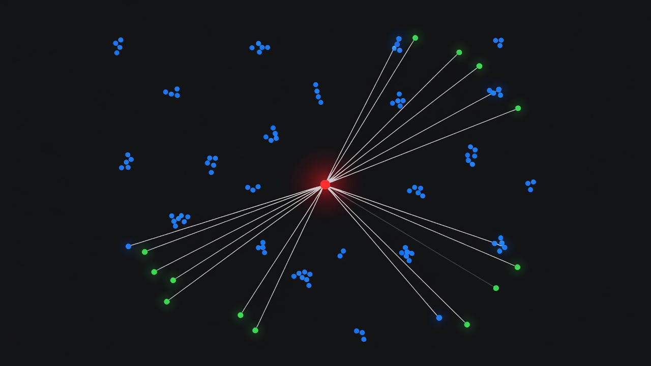
k-Nearest Neighbors (kNN)
k-Nearest Neighbors (kNN) classifies a query point by majority vote among its k most similar reference points in an embedding space. TarmacView uses kNN (k=10) ...
39 min read
Machine Learning
Classification
+3
FAISS (Facebook AI Similarity Search) is an open-source library for efficient similarity search and clustering of dense vectors, used by TarmacView to store and query approximately 9,000 labeled reference embeddings for nearest-neighbor surface quality classification. Covers index types (Flat, IVF, HNSW), cosine similarity via inner product on normalized vectors, GPU acceleration, and application to inspection image retrieval.
FAISS (Facebook AI Similarity Search) is an open-source C++ library developed by the Fundamental AI Research (FAIR) team at Meta for efficient similarity search and clustering of dense vectors. First released in 2017, FAISS has grown to over 40,000 GitHub stars and more than 5,200 citations of its GPU implementation paper. The FAISS packages have been downloaded more than 6 million times from Conda repositories. Major vector database companies including Zilliz (Milvus) and Pinecone either rely on FAISS as their core engine or have reimplemented FAISS algorithms in their production systems.
FAISS is purpose-built to address the computational challenge of finding nearest neighbors in high-dimensional vector spaces. The core operation is similarity search: given a query vector q, FAISS identifies the vectors in the reference set that are closest according to a specified distance metric. Formally, for a set of reference vectors {x₁, …, xₙ} in dimension d, FAISS efficiently computes j = argminᵢ ||q - xᵢ|| where ||·|| is the Euclidean distance. The library can also perform maximum inner product search argmaxᵢ ⟨q, xᵢ⟩ and supports additional metrics including L1, Linf, Canberra, Bray-Curtis, Jensen-Shannon, and Hamming distances through its IndexFlat and IndexHNSW implementations. FAISS returns not just the single nearest neighbor but the k nearest neighbors, supports batch processing of multiple queries simultaneously, and can execute range searches returning all elements within a given radius.
The library operates on dense vectors — fixed-length arrays of 32-bit floating-point numbers — that represent data points embedded in a continuous vector space. These vectors are typically generated by deep neural networks such as Vision Transformers (ViT), Convolutional Neural Networks (CNNs), or large language models. In modern machine learning pipelines, embeddings serve as intermediate representations that map complex input media into a vector space where locality encodes semantics. FAISS is the bridge between embedding extraction and downstream similarity-based tasks: it indexes the extracted embeddings and enables fast retrieval operations.
FAISS is extensively optimized for modern hardware architectures. On CPU, it leverages BLAS (Basic Linear Algebra Subprograms) libraries such as Intel MKL, OpenBLAS, or Apple Accelerate to perform fast matrix operations. It supports SIMD vectorization (SSE, AVX2, AVX-512) on x86 architectures and Neon intrinsics on ARM processors. On GPU, FAISS provides native CUDA implementations that can deliver 5–10x throughput improvements over CPU execution for typical workloads. The GPU implementation supports multiple GPUs in parallel, enabling distributed search across several devices simultaneously.
FAISS is not a vector database — it is a search library that can be embedded directly into applications. Unlike full database systems (Pinecone, Milvus, Qdrant, Weaviate), FAISS does not provide built-in persistence, replication, access control, concurrent write access, load balancing, sharding, transaction management, or query optimization. Instead, it exposes a clean C++ and Python API for building, querying, saving, and loading indexes. This intentional limitation to its scope allows FAISS to achieve maximum performance for the core nearest-neighbor search operation. The scope of the library is deliberately limited to Approximate Nearest Neighbor Search (ANNS) algorithmic implementation, and as the original FAISS paper states: “Faiss is not a database — it does not provide concurrent write access, load balancing, sharding, transaction management or query optimization.”
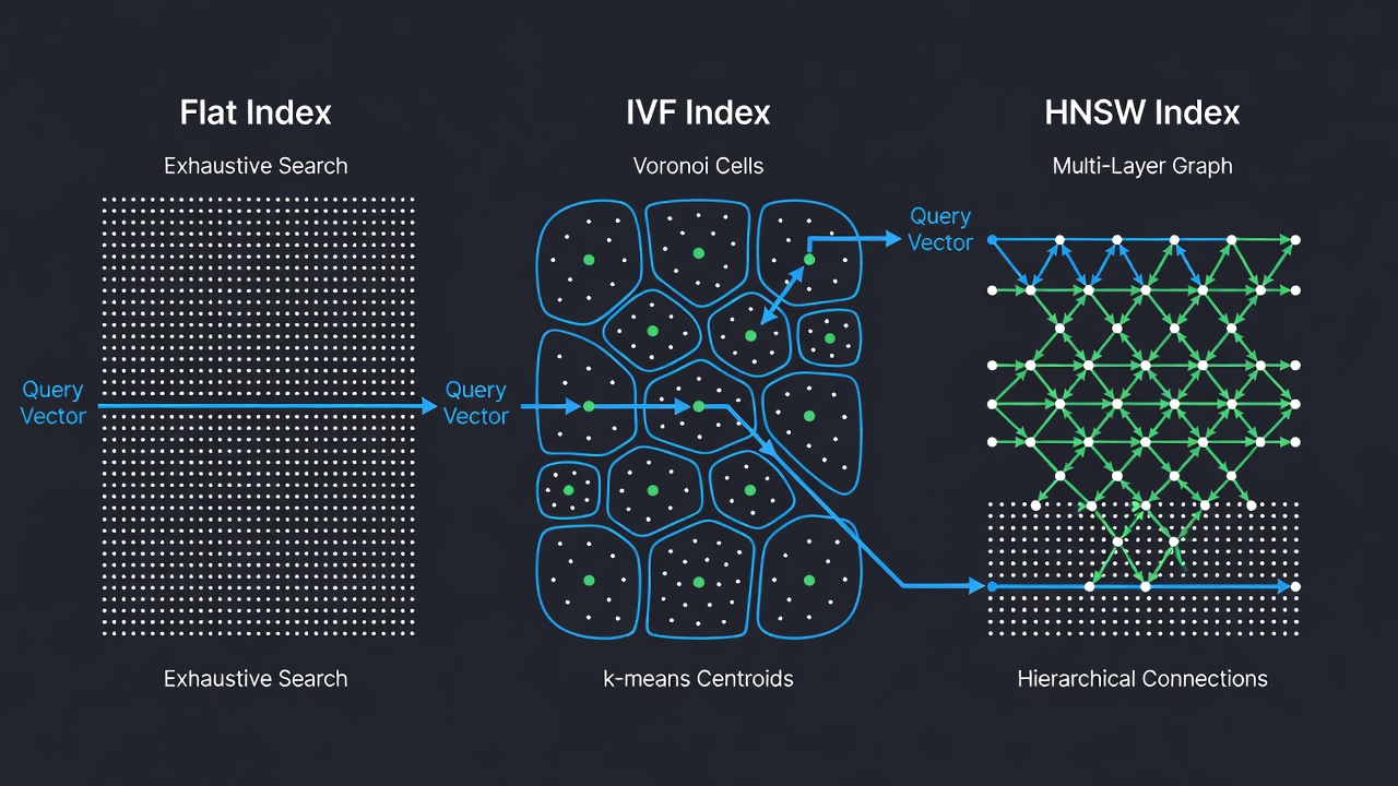
FAISS provides over twenty different index types, each designed for a specific combination of accuracy, speed, and memory trade-offs. The three most fundamental and widely used index types are IndexFlat (exact search), IndexIVF (inverted file with k-means clustering), and IndexHNSW (hierarchical navigable small world graph). Each index type is available with different distance metrics and encoded variants (e.g., FlatIP for inner product, FlatL2 for L2 distance). FAISS indexes can be composed hierarchically — for example, using HNSW as the coarse quantizer for an IVF index, yielding the IndexIVFPQ compound structure that powers billion-scale deployments.
IndexFlatIP is the simplest FAISS index. It stores all vectors in a flat array and performs an exhaustive brute-force search against every vector in the dataset. For each query, it computes the inner product between the query and every stored vector, then returns the indices and distances of the top-k results. This index is guaranteed to return the exact nearest neighbors — no approximations, no recall degradation. It is the only FAISS index that provides this guarantee; all other indexes are approximate and trade some recall for improved speed or reduced memory usage.
The computational complexity of IndexFlatIP is O(N × D) per query, where N is the number of reference vectors and D is the dimensionality. The index uses the highly optimized BLAS gemm (general matrix multiply) routine to compute all inner products in a single matrix multiplication. For a dataset of 100,000 vectors at 768 dimensions (a typical embedding size from DINOv2 ViT), a single query on CPU takes approximately 5–15 milliseconds depending on hardware and BLAS optimization. In batch mode with 1,000 queries, the index processes them all simultaneously using matrix-matrix multiplication, achieving significantly higher throughput than 1,000 individual queries.
IndexFlatIP serves a critical role in the FAISS ecosystem as the ground-truth oracle for evaluating approximate index accuracy. Practitioners build a flat index alongside their approximate index, run identical queries against both, and compute recall metrics. The standard FAISS benchmarking suite (faiss_benchmarks) uses this methodology to quantify the accuracy degradation of IVF, HNSW, and PQ indexes. In TarmacView, IndexFlatIP is used as the baseline reference for system validation, ensuring that approximate indexes used in production maintain acceptable recall.
The index is constructed with minimal code: index = faiss.IndexFlatIP(d) where d is the embedding dimensionality. Vectors are added with index.add(embeddings). Search is performed with index.search(query, k), which returns two float32 arrays: distances (shape [n_queries, k]) and indices (shape [n_queries, k], dtype int64). For inner product, larger distance values indicate greater similarity. The index requires no training step, as there are no parameters to learn — the vectors are stored and compared verbatim.
IndexIVFFlat is an approximate nearest-neighbor index that partitions the vector space into Voronoi cells using k-means clustering. The architecture is derived from the seminal “Video Google” paper by Sivic and Zisserman (ICCV 2003), which adapted text retrieval techniques to visual object matching. During indexing, the dataset is clustered into nlist clusters via k-means, and each vector is assigned to its nearest cluster centroid. The centroids are stored in a coarse quantizer (typically IndexFlatL2). During search, only vectors in the nprobe nearest clusters to the query are examined, dramatically reducing the number of distance computations required.
The speedup versus IndexFlatIP is approximately N / ((N / nlist) × nprobe) . With nlist=100 and nprobe=5, only 5% of the database is searched — queries that took 10ms on a flat index may complete in 0.5ms. However, the trade-off is recall degradation: some true nearest neighbors may fall outside the searched clusters and be missed. The k-means training step is critical for recall quality — the centroids must accurately represent the data distribution. FAISS requires the training set to contain at least 30 × nlist vectors for reliable centroid estimation.
Key parameters for IndexIVFFlat:
| Parameter | Description | Typical Range | Impact |
|---|---|---|---|
| nlist | Number of Voronoi cells (clusters) | 10 – 100,000 | Higher = finer partitioning, more memory for centroids, slower k-means training |
| nprobe | Number of cells searched at query time | 1 – 100+ | Higher = better recall (up to 99%), linearly slower search |
| metric | Distance metric (L2 or IP) | L2 or IP | Determines how distances are computed between vectors and centroids |
The nprobe parameter is especially important because it controls the search-time speed-accuracy trade-off without requiring index reconstruction. At query time, nprobe can be adjusted dynamically: set it to a high value (e.g., 20–50) during offline quality-critical operations where accuracy is paramount, and to a low value (e.g., 1–5) during high-throughput production runs where speed is prioritized. FAISS provides an auto-tuning mechanism (AutoTune) that searches over nprobe values to find the optimal configuration for a target recall.
Constructing an IndexIVFFlat requires a three-stage pipeline: training, adding, and searching. During training, k-means runs on a representative sample to learn cluster centroids. During adding, each database vector is assigned to its nearest centroid and appended to that centroid’s inverted list. During search, the query is compared against all centroids, the nprobe closest ones are selected, and only vectors in those selected lists are compared exhaustively. The factory string for IndexIVFFlat with inner product is "IVF100,Flat" where 100 is the nlist value. In Python: index = faiss.index_factory(d, "IVF100,Flat", faiss.METRIC_INNER_PRODUCT).
| Dataset size | Recommended nlist | Recommended nprobe | Expected recall | Speedup vs Flat |
|---|---|---|---|---|
| 10,000 | 10 – 100 | 1 – 5 | 95–98% | 5–20x |
| 100,000 | 100 – 1,000 | 5 – 20 | 95–99% | 20–100x |
| 1,000,000 | 1,000 – 10,000 | 10 – 50 | 95–99% | 100–500x |
| 10,000,000 | 10,000 – 100,000 | 20 – 100 | 90–98% | 500–5000x |
IndexHNSWFlat is a graph-based approximate nearest-neighbor index that constructs a multi-layer hierarchical graph known as a Navigable Small World. The algorithm, originally published by Malkov and Yashunin (2016), is inspired by the skip-list data structure. The index organizes vectors into layers: the bottom layer (layer 0) contains all vectors, and each subsequent layer contains a progressively smaller subset generated by a probabilistic level assignment. At insertion, each vector is assigned a level l = floor(-ln(uniform(0,1)) × mL) where mL = 1/ln(M). The entry point is at the highest existing layer, ensuring logarithmic graph traversal.
Search begins at the top layer (coarsest, with the fewest nodes) and descends through the layers, refining the candidate set at each step. At each layer, a greedy search traverses the graph toward the query by always moving to the neighbor that minimizes the distance. After finding the local minimum at the current layer, the algorithm descends to the next layer and repeats the process using the result from the layer above as the starting point. This hierarchical structure enables logarithmic search complexity O(log N), making HNSW one of the fastest approximate nearest-neighbor algorithms available for medium-to-large datasets.
The HNSW index has three critical parameters:
| Parameter | Description | Typical Range | Impact |
|---|---|---|---|
| M | Maximum number of bi-directional connections per node | 8 – 64 (default 32) | Higher M = more densely connected graph, better recall, more memory |
| efConstruction | Dynamic candidate list size during graph construction | 40 – 200 (default 40) | Higher = more thorough search during build, better quality graph, slower build |
| efSearch | Dynamic candidate list size during search | 10 – 200 (set at query time) | Higher = better recall, slower search (can tune without rebuild) |
The M parameter controls graph connectivity directly. Each vector maintains up to M bidirectional edges to its nearest neighbors. The graph uses a diversity-enforcing heuristic during neighbor selection: when a new node is added, its neighbor candidates are pruned to ensure diverse connectivity that avoids hub nodes dominating the graph structure. Higher M values produce more robust routing but increase memory consumption: approximately 4d + M × 2 × 4 bytes per vector for the graph structure plus vector storage.
The efConstruction parameter controls search thoroughness during index building. Larger values produce better-quality graphs but increase build time linearly. As a rule of thumb, efConstruction ≈ M × 2 provides a good balance for most workloads. The efSearch parameter is analogous to nprobe in IVF indexes — it controls search thoroughness at query time and can be adjusted dynamically without index reconstruction.
HNSW indexes offer several advantages over IVF indexes. They typically achieve higher recall at equivalent search speed, especially on high-dimensional data (d > 256). They do not require a separate training step (unlike IVF which needs k-means clustering, making HNSW suitable for dynamic datasets where vectors arrive incrementally). They exhibit graceful recall degradation as efSearch decreases — recall improves smoothly without sharp thresholds. However, HNSW indexes use more memory per vector (the graph adjacency lists add overhead) and are slower to build than IVF indexes. HNSW also does not natively support vector deletion, as removing nodes from the graph structure would compromise connectivity.
For TarmacView’s reference set of approximately 9,000 embeddings, an IndexHNSWFlat with M=32 and efSearch=64 achieves >99% recall at query times under 200 microseconds on CPU — a 50x speedup over IndexFlatIP with negligible accuracy loss. The factory string "HNSW32,Flat" constructs this index. In Python: index = faiss.index_factory(d, "HNSW32,Flat", faiss.METRIC_INNER_PRODUCT).
Cosine similarity measures the cosine of the angle between two non-zero vectors — it quantifies how similar two vectors are irrespective of their magnitude. The cosine similarity between vectors a and b is defined as cos(θ) = (a · b) / (||a|| × ||b||) where a · b is the dot product and ||a|| is the L2 norm of a. The result ranges from -1 (completely opposite direction) to +1 (identical direction), with 0 indicating orthogonality.
FAISS does not provide a dedicated cosine similarity metric. Instead, cosine similarity is implemented through a two-step transformation that the FAISS development team considers canonical. First, all vectors are L2-normalized to unit length — each vector is divided by its L2 norm so that ||a|| = 1 and ||b|| = 1. Second, METRIC_INNER_PRODUCT is used as the distance metric. For unit-normalized vectors, the inner product equals the cosine similarity: a · b = cos(θ). This equivalence follows directly from the cosine formula: when the denominator equals 1, the formula reduces to the dot product.
This normalization technique is standard across vector search systems because inner product is efficiently computable by highly optimized BLAS matrix multiplication routines. The computational cost of normalizing all vectors in the index is a one-time O(N × D) operation at index build time, and normalizing each query is O(D) — negligible compared to the cost of search itself. The L2 normalization is applied before vectors are added to the index and before queries are submitted, ensuring that all comparisons are in the cosine similarity space.
In FAISS, normalization is implemented using the IndexPreTransform wrapper combined with a NormalizationTransform (in Python, faiss.NormalizationTransform). The construction pattern is:
import faiss
import numpy as np

dimension = 768
# Create the inner product index
base_index = faiss.IndexFlatIP(dimension)
# Wrap with L2 normalization
index = faiss.IndexPreTransform(
    faiss.NormalizationTransform(dimension),
    base_index
)
# Vectors added here are automatically L2-normalized
index.add(reference_embeddings)
# Queries submitted here are automatically L2-normalized
distances, indices = index.search(query_embeddings, k)
Alternative approaches include manually normalizing vectors with faiss.normalize_L2() before adding and querying, or constructing the index via the index_factory which supports built-in normalization via the "L2norm" preprocessing step. With the factory method: index = faiss.index_factory(d, "L2norm,HNSW32,Flat") creates an index that automatically normalizes vectors to unit length before building the HNSW graph.
For TarmacView, this approach is essential because DINOv2 embeddings, like most Vision Transformer outputs, vary in magnitude across different images. Variations in exposure, lighting conditions, and camera settings during airport pavement inspection produce embeddings of different magnitudes even when capturing identical surface textures. Normalization removes the magnitude component and focuses similarity comparison on directional alignment — two surface images that capture the same pavement texture but at different exposure levels will register as highly similar because their normalized embeddings point in the same direction, even if their raw magnitudes differ significantly.
The FAISS FAQ explicitly addresses this: “The cosine similarity between vectors x and y is defined by cos(x, y) = ⟨x, y⟩ / (|x| × |y|). By normalizing query and database vectors beforehand, the problem can be mapped back to a maximum inner product search.” FAISS also notes that using inner product on normalized vectors is mathematically equivalent to using L2 distance on normalized vectors, with the relationship ||x - y||² = 2 - 2 × ⟨x, y⟩ for unit-normalized vectors.
The lifecycle of a FAISS index in production involves five distinct stages: configuration, training, population, serialization, and querying. Each stage has specific API calls, performance considerations, and best practices.
Configuration begins with selecting an index type and distance metric. FAISS provides the factory string mechanism — a compact string specification that constructs complex indexes. The factory pattern is the recommended approach because it abstracts away the specific class hierarchy and automatically selects the optimal implementation:
| Factory String | Index Type | Memory per Vector (d=768) | Use Case |
|---|---|---|---|
"Flat" | IndexFlat (exact L2 search) | 3,072 bytes | Small reference sets, ground truth |
"IVF100,Flat" | IndexIVFFlat with 100 centroids | ~3,100 bytes | Medium sets, fast approximate search |
"HNSW32,Flat" | IndexHNSWFlat with M=32 | ~3,328 bytes | Fast approx search, dynamic data |
"IVF100,PQ16" | IndexIVFPQ, 16 sub-vectors | ~80 bytes | Large-scale, memory-constrained |
"IVF100,SQ8" | IndexIVF with scalar quantization | ~784 bytes | Balanced, excellent speed |
Training is required only for indexes that learn a data distribution (IVF, PQ, SQ, etc.). During training, the index runs k-means clustering on a representative sample of vectors. For the k-means algorithm, FAISS uses multiple random initializations and selects the one with the lowest distortion. The training set should be representative of the data that will be indexed — using a random subset of 1–10% of the full dataset is common practice. FAISS requires training vectors to be the same dimensionality as the data that will be indexed. The index.is_trained flag indicates whether training has been completed. The training call is: index.train(training_vectors). For datasets where the index has already been trained (e.g., pre-trained centroids are loaded from a file), calling train again is unnecessary and will overwrite the learned parameters.
Population adds vectors to the trained index: index.add(reference_vectors). The ntotal property tracks the number of vectors added. For IVF indexes, each vector is assigned to its nearest cluster centroid and appended to that centroid’s inverted list during the add operation. For HNSW indexes, the graph is incrementally built: each new vector is assigned a layer level, and edges are established to its M nearest neighbors at each layer using the efConstruction parameter. Adding vectors is typically slower than querying, especially for HNSW where the graph must be updated.
Serialization saves the index to disk: faiss.write_index(index, "index.faissindex"). The index is loaded back with index = faiss.read_index("index.faissindex"). Serialization preserves the complete index state including trained centroids, graph structure, all stored vectors, distance metric configuration, and internal parameters. The standard file extension is .faissindex. Serialization size depends on index type and vector count — for IndexFlat with N vectors of dimensionality D, the size is approximately N × D × 4 bytes plus small overhead.
Querying retrieves the k nearest neighbors: distances, indices = index.search(query_vectors, k). The distances array contains similarity or distance values depending on the metric. The indices array contains the positions of the matching reference vectors as they were added (0-indexed). For batch queries, FAISS efficiently processes multiple queries simultaneously using matrix-matrix multiplication, achieving significantly better throughput than individual query-at-a-time calls. The index objects are thread-safe for search operations on separate index instances, enabling parallel query serving in production deployments.
FAISS is frequently used to implement k-Nearest Neighbors (kNN) classification — a non-parametric machine learning method that classifies a query point based on the majority label among its k nearest neighbors in the reference set. This approach is particularly attractive when: (1) the reference set is regularly updated with new labeled samples, (2) the embedding space captures meaningful semantic relationships between data points, and (3) interpretable, instance-based decisions are preferred over black-box neural classifiers.
The classification pipeline using FAISS follows five steps:
Build a labeled reference set: Each reference vector is paired with a ground-truth label (e.g., “asphalt - good condition”, “concrete - surface cracked”, “tarmac - patched”). The labels are stored in a separate array aligned with the FAISS index order. TarmacView maintains approximately 9,000 such labeled reference embeddings spanning multiple surface types and quality conditions.
Index the reference vectors: All reference embeddings are added to a FAISS index. For exact search with perfect recall, IndexFlatIP is used. For approximate search at scale, IndexHNSWFlat or IndexIVFFlat provide sub-millisecond query times with >99% recall when properly tuned.
Submit query embeddings: For each new image to classify, extract its embedding using the same embedding model (DINOv2 with 768-dimensional output) and normalize to unit length for cosine similarity.
Retrieve k nearest neighbors: FAISS returns the indices and distances of the k most similar reference vectors. The k parameter controls the bias-variance trade-off. Smaller k (e.g., 3–5) produces decision boundaries sensitive to local structure but prone to overfitting noise. Larger k (e.g., 15–20) produces smoother boundaries with better generalization but may lose fine-grained distinctions. TarmacView uses k=10, balancing robustness against outliers with sensitivity to subtle surface quality variations.
Perform majority voting: Count the labels among the k neighbors and select the most frequent label as the classification result. Optionally, distance-weighted voting assigns higher weight to closer neighbors: weight = 1.0 / (distance + ε) where ε is a small constant to prevent division by zero. Weighted voting is particularly beneficial when the reference set has uneven class distributions or when neighbor density varies across the embedding space.
| k value | Bias | Variance | Best for |
|---|---|---|---|
| 1 – 3 | Low | High | Large, clean reference sets, fine-grained boundaries |
| 5 – 10 | Moderate | Moderate | Balanced, general-purpose classification |
| 15 – 30 | Higher | Lower | Noisy labels, smooth decision boundaries |
The distance scores returned by FAISS also inform confidence estimation. If the top-k neighbors all share the same label and have high similarity scores (cosine similarity > 0.95), the classification is highly confident. If the vote is split (e.g., 6 out of 10 for the winning label) or similarity scores are low (< 0.70), the system can flag the result for human review. This confidence-aware architecture is critical for safety-critical applications like airport pavement inspection, where misclassification could affect maintenance prioritization and operational safety.
The embedding contract between the DINOv2 model and the FAISS index is fundamental to classification accuracy. The embedding extractor is trained via self-supervised learning so that distances between embeddings reflect visual similarity between pavement surface images. The FAISS index faithfully retrieves nearest neighbors according to the cosine similarity metric. When this contract holds — when visually similar surface conditions produce nearby embeddings — the kNN classification achieves high accuracy with the inherent interpretability of showing exactly which reference images informed each classification decision.
FAISS GPU support is a first-class feature that provides substantial performance improvements for both index construction and search. The GPU implementation, described in the paper “Billion-scale similarity search with GPUs” (Johnson, Douze, Jégou, 2017), is written in CUDA C++ and leverages NVIDIA GPU architectures from Kepler (Compute Capability 3.5) through Hopper (Compute Capability 9.0+) and beyond.
FAISS GPU acceleration delivers measurable performance improvements: 5–10x search throughput improvement over CPU for typical IVF and HNSW indexes; up to 12x faster index building for IVF indexes since k-means clustering is highly parallelizable; 8x lower latency for HNSW queries on GPU using optimized graph traversal kernels; and native support for batched queries where GPUs excel at processing hundreds or thousands of queries simultaneously through matrix-matrix operations.
The GPU implementation covers the most commonly used index types through dedicated CUDA classes:
| GPU Index Class | CPU Equivalent | CUDA Features Used |
|---|---|---|
| GpuIndexFlat | IndexFlat | BLAS gemm on GPU, shared memory tiling |
| GpuIndexIVFFlat | IndexIVFFlat | Parallel distance computation, warp-level reductions |
| GpuIndexIVFPQ | IndexIVFPQ | PQ lookup tables on GPU, fast code assignment |
| GpuIndexIVFScalarQuantizer | IndexIVFScalarQuantizer | float16 support on Pascal+ GPUs |
The GPU implementation uses warp shuffles (available on Compute Capability 3.0+) and read-only texture caching via ld.nc / __ldg (Compute Capability 3.5+). The k-selection algorithm — finding the top-k values from a large array of distances — operates at up to 55% of theoretical peak GPU performance, enabling a nearest neighbor implementation 8.5x faster than prior GPU state-of-the-art according to the 2017 paper. For GPU memory management, a StandardGpuResources object allocates scratch space on GPU: approximately 512 MiB on GPUs with ≤4 GiB memory, and approximately 1,536 MiB on larger GPUs. This scratch space avoids repeated cudaMalloc / cudaFree calls during search.
FAISS provides seamless CPU-GPU interoperability through two key functions: faiss.index_cpu_to_gpu(cpu_index, device_id) transfers a CPU index to a specified GPU device, and faiss.index_gpu_to_cpu(gpu_index) transfers a GPU index back to CPU memory. For multi-GPU deployments, faiss.index_cpu_to_gpu_multiple_py(resources, cpu_index) distributes an index across all available GPU devices, and queries are automatically load-balanced. The multi-GPU approach can scale to indexes containing hundreds of millions of vectors by partitioning across GPU memory spaces.
| Scenario | CPU | GPU (1x) | GPU (8x) |
|---|---|---|---|
| IndexFlat search (100K x 768d), batch=8192 | 50 ms | 5 ms | <1 ms |
| IVF k-means training (1M x 128d), nlist=1000 | 120 s | 10 s | 5 s |
| HNSW build (100K x 128d), M=32 | 30 s | 8 s | — |
| Billion-scale k-NN graph | days | 12 hours | 4 hours |
For TarmacView, GPU acceleration is valuable during the index construction phase when new reference images are added periodically. Building an IVF index with k-means on 9,000 768-dimensional vectors completes in approximately 1–2 seconds on a modern GPU (NVIDIA A100 or RTX 4090) versus 30–60 seconds on CPU. During inference, the index remains on CPU for cost-effective deployment — query latency on CPU with IndexHNSWFlat is already under 200 microseconds for the 9K reference set, and converting to GPU would add PCIe transfer overhead without meaningful latency benefits.

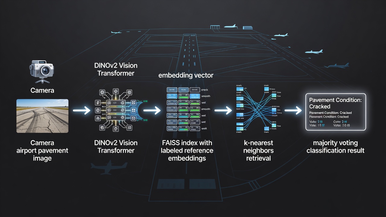
TarmacView integrates FAISS as the core similarity search engine for its automated airport pavement surface quality classification system. The system classifies pavement surface types (asphalt, concrete, tarmac) and surface quality conditions (good, fair, poor, distressed, cracked, patched) by comparing inspection images against a curated reference set of approximately 9,000 labeled embeddings.
Reference Set Construction: Each reference embedding is extracted from a high-resolution pavement image using a DINOv2 Vision Transformer model (ViT-B/14 or equivalent), which produces a 768-dimensional vector capturing visual features such as texture patterns, color distribution, crack morphology, aggregate exposure, surface wear, and repair evidence. Each embedding is annotated with ground-truth labels established by certified pavement inspectors during an initial system training phase. The reference set spans multiple airports, climate zones, and pavement ages to ensure robust classification across diverse conditions.
Index Selection: TarmacView chooses the index type based on deployment requirements:
| Deployment Scenario | Index Type | Query Time | Recall | Memory |
|---|---|---|---|---|
| Offline QA / validation | IndexFlatIP | ~2 ms | 100% | ~28 MB |
| Real-time field deployment | IndexHNSWFlat (M=32, efSearch=64) | <200 μs | >99% | ~30 MB |
| Edge device (limited RAM) | IndexIVFFlat (nlist=100, nprobe=10) | ~300 μs | ~97% | ~28 MB |
Classification Workflow:
A drone-mounted camera (e.g., DJI Matrice series with high-resolution payload) or handheld inspection device captures pavement images during routine airport airfield inspections, following ICAO Annex 14 and FAA AC 150/5380-7B guidelines for pavement condition assessment.
Each image is preprocessed (cropped to remove non-pavement areas, normalized to standard resolution) and passed through the DINOv2 embedding model hosted on an edge inference accelerator (NVIDIA Jetson or equivalent).
The resulting 768-dimensional embedding is L2-normalized to unit length for cosine similarity computation. The normalization ensures that exposure variations between inspection flights do not affect similarity ranking.
FAISS queries the IndexHNSWFlat index with k=10, returning the 10 nearest reference embedding indices and their inner product similarity scores (equivalent to cosine similarity for normalized vectors).
The system performs majority voting on the labels of the 10 neighbors. If the winning label has at least 6 of 10 votes (60% consensus), the classification is accepted with a confidence score computed as the ratio of winning votes to total votes.
If the vote is split below 60% consensus, the image embedding and top-10 reference images are flagged for human review by a certified pavement inspector through the TarmacView web interface.
Classifications are recorded in the TarmacView database with timestamps, GPS coordinates, surface type, quality condition, confidence score, and links to the supporting reference images. This creates a fully auditable inspection trail for regulatory compliance.
This FAISS-powered classification pipeline enables TarmacView to process thousands of pavement images per day with consistent, objective quality assessment — reducing reliance on subjective human visual inspection and enabling scalable airport airfield condition monitoring across entire airport networks.
FAISS occupies a distinct niche in the vector search ecosystem. It is a library, not a database, and this distinction has significant implications for architecture, deployment, and operational characteristics. The FAISS library provides pure nearest-neighbor search functionality without the overhead of a full database management system.
| Feature | FAISS | Pinecone | Milvus | Qdrant | Weaviate |
|---|---|---|---|---|---|
| Type | Library | Managed service | Database | Database | Database |
| Deployment | Embedded | Cloud / SaaS | Self-hosted / Cloud | Self-hosted / Cloud | Self-hosted / Cloud |
| Persistence | Manual save/load | Automatic | Automatic | Automatic | Automatic |
| CRUD | Not built-in | Full CRUD | Full CRUD | Full CRUD | Full CRUD |
| Metadata filtering | ID-based only | Rich filters | Attribute + scalar | Payload filtering | Graph-based |
| Scaling | Manual sharding | Auto-scaling | Distributed Raft/Paxos | Distributed | Distributed |
| GPU support | Native CUDA | No | Limited (CUDA) | No | No |
| Query latency | 10 μs – 1 ms | 2 – 10 ms | 1 – 10 ms | 1 – 5 ms | 1 – 10 ms |
| License | MIT | Proprietary | Apache 2.0 | Apache 2.0 | BSD-3 |
The key advantage of FAISS over full database systems is performance and simplicity. FAISS queries are typically 10–100x faster than equivalent queries on database systems because: the library runs in-process without network round-trips; there is no query parsing, authentication, or authorization overhead; there is no storage engine indirection or buffer pool management; and FAISS indexes are optimized linear algebra data structures with no transactional overhead. FAISS operates directly on in-memory data structures using optimized BLAS routines, with no inter-process communication.
The key advantage of database systems over FAISS is operational convenience. They provide automatic data durability with write-ahead logging and replication, support rich metadata filtering (e.g., “find similar images captured after January 2025 that show concrete pavement in the US Southwest region”), offer REST or gRPC APIs for language-agnostic access, include monitoring dashboards and alerting, and handle backup and disaster recovery. They support concurrent read and write operations with transaction guarantees and schema evolution.
For TarmacView, using FAISS directly rather than a vector database is the correct architectural choice for four reasons: (1) the reference set is small (~9K vectors, approximately 28 MB) and fits entirely in memory; (2) query latency requirements are aggressive (sub-200 microsecond classification is achievable with HNSW on CPU); (3) the system runs in edge deployments at airports where network access to a database server may be impractical or introduce unacceptable latency; and (4) the index is rebuilt infrequently (weekly or monthly as new reference images are added after inspector validation), making manual serialization and version control manageable.
FAISS index serialization converts an in-memory index object to a binary representation that can be saved to disk, transferred over a network, or loaded into a different process or machine. Serialization preserves the complete index state including all stored vectors, trained centroids (for IVF and PQ indexes), graph structure (for HNSW), distance metric configuration (L2 vs IP vs other), and all internal parameters (efConstruction, M, normalization settings, etc.).
The primary serialization functions are:
| Function | Description | Output | Use Case |
|---|---|---|---|
| write_index(index, filename) | Writes index to file | .faissindex file | Persistent disk storage |
| read_index(filename) | Loads index from file | Index object | Load for serving |
| serialize_index(index) | Writes index to bytes | Python bytes object | Database storage, message queues |
| deserialize_index(data) | Loads index from bytes | Index object | Load from memory buffer |
Serialization size depends on index type and vector count. For IndexFlatIP with N vectors of dimension D, the file size is approximately N × D × 4 bytes (32-bit float storage) plus overhead for the header and metadata. For IndexIVFFlat, additional storage is consumed by cluster centroids: nlist × D × 4 bytes. For IndexHNSWFlat, the graph structure adds N × M × 2 × 4 bytes for the adjacency lists (assuming 32-bit neighbor indices stored bidirectionally). For TarmacView’s HNSW index with 9,000 vectors at 768 dimensions and M=32, the serialized file is approximately 25 MB: 9,000 × 768 × 4 = 27.6 MB for vectors plus 9,000 × 32 × 2 × 4 = 2.3 MB for graph structure, minus the fact that HNSW stores vectors in a flat index internally.
Serialization supports cross-context transfer: an index built on GPU can be saved to disk and loaded on CPU. The recommended pattern is to always transfer GPU indexes to CPU before serialization:
cpu_index = faiss.index_gpu_to_cpu(gpu_index)    # transfer to CPU
faiss.write_index(cpu_index, "production_index.faissindex")  # save to disk

# On a different machine (or later):
deployed_index = faiss.read_index("production_index.faissindex")
deployed_index.hnsw.efSearch = 64    # set search-time parameters
D, I = deployed_index.search(queries, k)
For production deployments, the serialized index can be version-controlled alongside application code. TarmacView maintains versioned FAISS index files in its deployment artifacts, ensuring that every edge deployment uses an identical reference set for reproducible classification results. When new reference images are added and validated, a new index is trained, its accuracy is benchmarked against the previous index using the ground-truth IndexFlatIP, and the new index is deployed through the standard CI/CD pipeline.
While TarmacView’s current reference set of approximately 9,000 vectors is modest, FAISS is engineered to scale to billions of vectors on a single server. The library provides a comprehensive toolkit for handling large-scale deployments through three complementary techniques: vector compression, non-exhaustive search, and distributed indexing.
Product Quantization (PQ) is a lossy compression technique that dramatically reduces per-vector memory footprint. PQ splits each D-dimensional vector into m sub-vectors of equal size (D/m dimensions each). Each sub-vector is quantized independently using a codebook of 256 entries (8 bits) learned via k-means clustering. The original float32 vector (4 × D bytes) is compressed to m bytes of code indices plus a small codebook. PQ compression ratios of 4x to 16x are common, enabling a single machine to index hundreds of millions of vectors in main memory. FAISS IndexIVFPQ combines IVF with PQ, using the cluster centroids as a coarse quantizer and PQ codes for residual compression. The distance computation uses Asymmetric Distance Computation (ADC): the query remains uncompressed, and distances to PQ-compressed database vectors are computed via precomputed lookup tables, avoiding decompression overhead.
| PQ Configuration | Bytes/vector (d=768) | Memory, N=100M | Recall vs uncompressed |
|---|---|---|---|
| PQ32 (m=32, 8-bit) | 40 | 3.7 GB | ~90-95% |
| PQ64 (m=64, 8-bit) | 72 | 6.7 GB | ~95-98% |
| PQ96 (m=96, 8-bit) | 104 | 9.7 GB | ~97-99% |
Scalar Quantization (SQ) converts each float32 component to an 8-bit or 4-bit unsigned integer, reducing storage by 4x (SQ8) or 8x (SQ4) with minimal accuracy loss. The factory string "IVF100,SQ8" creates an IVF index with scalar quantization. SQ is faster than PQ at query time because distance computations are performed directly on the quantized values without lookup table precomputation. SQ8 stores one byte per dimension; SQ4 stores two dimensions per byte.
For billion-scale datasets, the recommended FAISS configuration combines HNSW as the coarse quantizer with IVFPQ for vector compression: quantizer = IndexHNSWFlat(d, hnsw_m); index = IndexIVFPQ(quantizer, d, nlist, M, nbits). The HNSW quantizer accelerates centroid lookup compared to flat search during query time, and PQ compresses database vectors to a fraction of their original size. The original FAISS paper (2017) benchmarked building a k-NN graph on 95 million images (from the YFCC100M dataset) in 35 minutes on GPUs, and a k-NN graph on 1 billion vectors in under 12 hours on 4x Maxwell Titan X GPUs.
FAISS IndexShards splits a large dataset across multiple sub-indexes, each on potentially different machines or GPUs. Each shard receives a subset of the vectors and processes queries independently. Results are merged via a k-way merge of the top-k results from each shard. This approach provides linear scaling with the number of available servers: doubling the shard count halves the search time for a fixed dataset size.
For datasets exceeding available RAM, FAISS provides on-disk indexes that keep the index structure (inverted lists or graph) in memory but store vector data on SSD. The IndexOnDisk class and related utilities transparently load vector data from disk during search, using memory-mapped files or explicit I/O operations. With modern NVMe SSDs providing 3–7 GB/s sequential read speeds, on-disk search can approach in-memory performance for many workloads, especially when spatial locality (neighboring vectors stored contiguously on disk) is maintained.
For TarmacView, the current 9K reference set is well within FAISS’s optimal range for exact search with IndexFlatIP. However, as the system expands to include reference images from hundreds of airports and multiple inspection campaigns — potentially growing to millions of labeled embeddings — FAISS’s scaling mechanisms (IVF for non-exhaustive search, PQ for compression, on-disk storage for out-of-RAM datasets) provide a clear upgrade path without requiring a fundamentally different architecture. The index type can be upgraded from IndexFlatIP → IndexIVFFlat → IndexIVFPQ → IndexShards(IndexIVFPQ) as the reference set grows, with each step trading minimal accuracy for order-of-magnitude improvements in search speed and memory efficiency.
The FAISS literature (including the comprehensive 2024 arXiv paper “The Faiss Library” by Douze, Guzhva, Deng, Johnson, Szilvasy, Mazaré, Lomeli, Hosseini, and Jégou) provides detailed guidance on index selection: “There exists a choice between a dozen index types, and the optimal one usually depends on the problem’s constraints.” FAISS also includes a comprehensive benchmarking suite (faiss_benchmarks) that measures recall and throughput across different index configurations, running searches with ground-truth results from IndexFlat to quantify accuracy. Practitioners are encouraged to benchmark their specific data distribution — the optimal index for a given dataset depends on vector dimensionality, dataset size, target recall, latency budget, and available memory.
Leverage FAISS for high-performance similarity search on your image embedding data. Contact us to learn how TarmacView integrates FAISS for real-time surface quality classification and inspection image retrieval.
k-Nearest Neighbors (kNN) classifies a query point by majority vote among its k most similar reference points in an embedding space. TarmacView uses kNN (k=10) ...
DINOv3 (self-DIstillation with NO labels v3) is a self-supervised vision transformer (ViT-B/16) pretrained on 1.7 billion images, producing high-quality 768-dim...
An embedding space is a high-dimensional mathematical space in which objects such as images, text, or sensor data are represented as vectors, enabling similarit...