FWD Deflection Data Analysis and Back-Calculation

Deflection Basin Interpretation

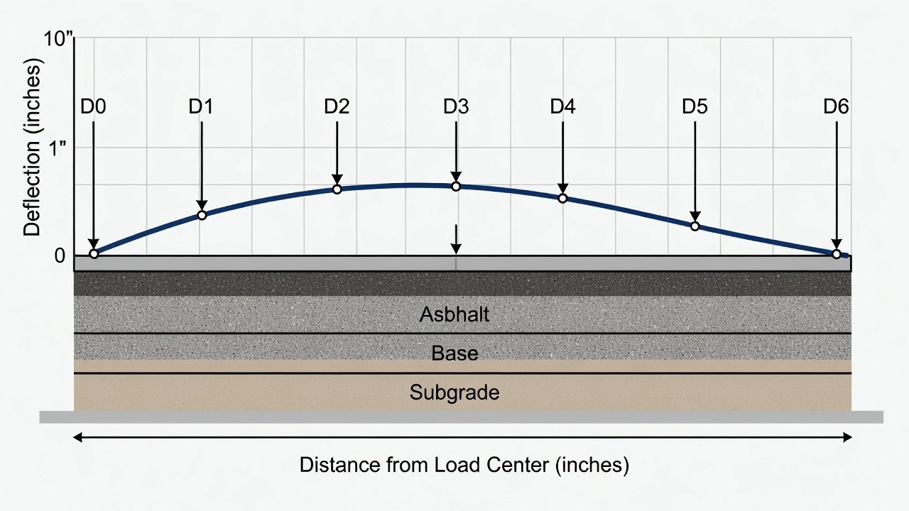
The deflection basin is the bowl-shaped depression in the pavement surface created by the impulse load from the Falling Weight Deflectometer (FWD). A standard FWD test employs seven geophone sensors positioned at radial distances of 0, 12, 24, 36, 48, 60, and 72 inches (0, 305, 610, 914, 1219, 1524, and 1829 mm) from the center of the loading plate, which has a radius of 5.9 inches (150 mm). The sensors record peak vertical surface deflection at each location in response to an impulse load typically ranging from 9,000 to 16,000 lbf (40 to 71 kN) with a pulse duration of 25 to 30 milliseconds, simulating the loading characteristics of a single heavy truck axle moving at moderate speed.

The deflection at the center of the load plate (D0) is the maximum deflection and is influenced primarily by the stiffness of the surface layer (asphalt concrete or Portland cement concrete) and the overall structural capacity of the pavement system. A D0 value below 0.005 inches (0.13 mm) at a 9,000 lbf (40 kN) load typically indicates a very stiff pavement in good structural condition, while D0 exceeding 0.020 inches (0.51 mm) indicates a structurally weak pavement that may require rehabilitation. The Impulse Stiffness Modulus (ISM) , calculated as ISM = Load / D0 (in kN/mm or kip/in), provides the simplest single-parameter structural indicator. ISM values below 50 kN/mm (285 kip/in) generally indicate structural deficiency, while values above 100 kN/mm (570 kip/in) indicate adequate structural capacity. The AASHTO 1993 Guide relates ISM to the effective structural number (SN_eff) through empirical correlations specific to each agency’s pavement types.

The Area parameter quantifies the shape of the deflection basin and is computed as Area = (1/2D0) × [D0 + 2(D1 + D2 + … + Dn-1) + Dn] × Δr, where Δr is the sensor spacing interval (typically 12 inches or 305 mm). The Area parameter provides insight into the relative stiffness distribution between layers. Area values below 20 inches indicate that the HMA layer is thin or weak relative to the underlying base and subgrade — the deflection basin is narrow and concentrated near the load center. Area values between 22 and 28 inches indicate a balanced structural section where the HMA, base, and subgrade are contributing proportionally to load distribution. Area values above 30 inches indicate a thick HMA layer or a stiff surface layer over a weaker subgrade — the basin is widely distributed because the stiff surface spreads the load over a large area, reducing subgrade stress but potentially hiding a weak foundation.

The deflection ratios (D1/D0, D2/D0, D4/D0, D7/D0) provide additional diagnostic information about individual layer condition. A high D1/D0 ratio (approaching 0.9) combined with a rapidly decreasing basin suggests the HMA layer is the primary load-carrying element with relatively weak support from underlying layers. A high D4/D0 or D7/D0 ratio (exceeding 0.3) indicates a weak subgrade that is deflecting significantly even at large distances from the load center, because the stress bulb extends deep into the subgrade at those sensor positions. The Surface Curvature Index (SCI) , defined as SCI = D0 - D2 (or sometimes SCI = D0 - D1), is a measure of surface layer condition. SCI values typically range from 0.001 to 0.015 inches (0.025 to 0.381 mm), with higher values indicating weaker or thinner surface layers. The Base Damage Index (BDI = D2 - D4) and Base Curvature Index (BCI = D4 - D7) provide similar diagnostics for the base and subgrade layers respectively.

Standard FWD testing procedures according to ASTM D4694 (Standard Test Method for Deflections with a Falling Weight-Type Impulse Load Device) require a minimum of four seating drops at each test location to ensure proper plate contact with the pavement surface, followed by three recording drops at one or more load levels. The deflections are typically normalized to a standard load of 9,000 lbf (40 kN) for highway pavements or 40,000-54,000 lbf (178-240 kN) for airport pavements using Heavy Weight Deflectometer (HWD) equipment. Temperature effects on the asphalt concrete modulus are significant — the measured deflection of an HMA pavement can be 2 to 3 times higher at 95°F (35°C) than at 50°F (10°C) due to the viscoelastic nature of asphalt. All FWD deflections must be temperature-corrected to a standard reference temperature, typically 68°F (20°C), before back-calculation, using temperature correction models specific to the local HMA mix design.

Back-Calculation Concept

Back-calculation is the inverse analysis process that determines the elastic modulus of each pavement layer from the measured deflection basin. The fundamental problem is: given the measured surface deflections at 7 sensor positions, the known layer thicknesses (from cores or construction records), the known load magnitude and plate geometry, and the Poisson’s ratio of each layer (typically 0.35 for HMA, 0.35-0.40 for granular base, 0.40-0.50 for subgrade), determine the elastic modulus (E) of each layer that produces the best match between calculated and measured deflections.

This is not a direct solution — there is no closed-form equation that gives layer moduli from deflections. Back-calculation is an iterative optimization problem solved by the following process:

Step 1 — Forward model selection. A layered elastic analysis (LEA) program is selected as the forward engine. The most common forward engines are WESLEA (developed by the U.S. Army Corps of Engineers Waterways Experiment Station), BISAR (developed by Shell), ELSYM5, and LEAF (developed by the FAA for airport pavements). All are based on Burmister’s layered elastic theory — an extension of Boussinesq’s solution for a homogeneous half-space to a system of horizontal layers with different elastic properties. The forward model computes stresses, strains, and deflections in a multilayered elastic system given the load, geometry, and material properties. The key assumptions are: each layer is homogeneous, isotropic, and linearly elastic; layers extend infinitely in the horizontal direction; the subgrade extends infinitely downward; and the interface between layers is either fully bonded (no slip) or fully unbonded (no shear transfer).

Step 2 — Seed modulus estimation. Initial estimates (seed moduli) are assigned to each layer. Typical seed values for highway pavements are: HMA surface = 300,000 to 500,000 psi (2,070 to 3,450 MPa); granular base = 20,000 to 50,000 psi (138 to 345 MPa); subbase = 10,000 to 25,000 psi (69 to 172 MPa); subgrade = 5,000 to 15,000 psi (34 to 103 MPa). Seed moduli can also be estimated from the ISM or from the Boussinesq equation applied to the outer sensor deflection (D7), which is primarily influenced by the subgrade modulus. Poor seed moduli increase the number of iterations required for convergence and increase the risk of convergence to a local minimum — a non-unique solution that satisfies the error criteria but does not represent the true layer moduli.

Step 3 — Forward computation. The forward elastic program computes the theoretical deflection basin using the seed moduli, known layer thicknesses, Poisson’s ratios, load magnitude, and plate geometry. The output is a set of computed deflections at each sensor position (D0_calculated through D7_calculated).

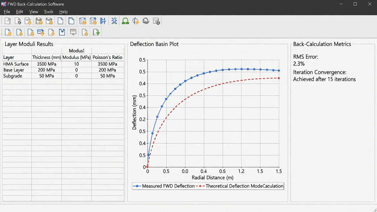
Step 4 — Error computation. The difference between measured and computed deflections is quantified using the Root Mean Square (RMS) error or the Sum of Absolute Error (SAE) . The most widely used metric is: RMS(%) = (1/nd) × Σ[(dci - dmi)/dmi]² × 100 where nd is the number of deflection sensors, dci is the computed deflection at sensor i, and dmi is the measured deflection at sensor i. An RMS error below 1% is considered excellent, 1-2% is acceptable for most purposes, and above 2% may indicate incorrect layer structure assumptions, poor seed moduli, or nonlinear material behavior not captured by the linear elastic model.

Step 5 — Optimization. If the RMS error exceeds the target tolerance (typically 1-2%), the optimization algorithm adjusts the layer moduli and returns to Step 3. The optimization methods differ between software packages. EVERCALC uses the Gauss-Newton nonlinear least squares (NLS) method, which computes the Jacobian matrix (sensitivity of each deflection to each modulus) and uses a Taylor series expansion to find the optimal step direction and magnitude. MODULUS uses the Hookes-Jeeves pattern search algorithm, which evaluates the error surface using a grid of modular ratios and then converges to the minimum through iterative exploration and pattern moves. The optimization is constrained by user-specified minimum and maximum modulus values for each layer to prevent convergence to physically unrealistic values.

Step 6 — Convergence check and validation. After convergence, the software outputs the final moduli with RMS error. The analyst must validate the results by checking: (1) RMS error is within acceptable range; (2) back-calculated moduli are within typical ranges for the material types; (3) moduli vary smoothly along the project rather than exhibiting erratic station-to-station swings; (4) layer compensation is not occurring — a condition where errors in one layer’s modulus are compensated by unrealistic adjustments in another layer’s modulus; (5) the solution is physically reasonable based on local experience with similar pavement structures.

The back-calculation problem is inherently non-unique — multiple combinations of layer moduli can produce the same deflection basin, particularly when the number of unknown layers exceeds 3 or when layer thicknesses are not accurately known. This is why: accurate layer thickness information from cores or ground-penetrating radar (GPR) is essential; the subgrade modulus is typically the most reliably determined parameter because it is constrained by the outer sensors; the HMA modulus is the most sensitive to temperature and should be normalized to a reference temperature; and the base modulus is often the most uncertain parameter because its contribution to the deflection basin overlaps with the HMA and subgrade contributions.

Back-Calculation Software

Five major software programs are used for FWD deflection data analysis and back-calculation, each with distinct theoretical approaches, capabilities, and application domains.

MODULUS — Texas Transportation Institute

MODULUS is a public-domain back-calculation system developed by the Texas Transportation Institute (TTI) for the Texas Department of Transportation (TxDOT). The current version is MODULUS 6.0 for Windows (released October 2001), succeeding DOS versions dating back to the late 1980s. MODULUS uses a fundamentally different approach from most back-calculation programs — the database pattern-matching method rather than iterative optimization per bowl. Before any back-calculation, MODULUS pre-computes a database of deflection bowls using WESLEA as the forward engine for a grid of modular ratio combinations (E_surface/E_subgrade, E_base/E_subgrade, E_subbase/E_subgrade). For a 4-layer system, this requires 3×3×3 = 27 combinations, which are computed once per pavement structure. During back-calculation of individual deflection bowls, MODULUS first solves for the subgrade modulus directly using the relationship between the bowl shape and sensor positions, then uses the Hookes-Jeeves pattern search algorithm to refine the modular ratios for the upper layers. This approach is extremely fast — approximately 5 seconds per bowl on older hardware — because the forward computations are pre-computed in the database rather than performed iteratively for each bowl. MODULUS also includes a convexity test that evaluates whether the solution represents a true global minimum, and a depth-to-bedrock estimation capability using the Rohde/Scullion regression method. MODULUS supports a maximum of 4 pavement layers plus a rigid (bedrock) layer and is limited to flexible pavements only. It includes AASHTO-compliant subsectioning into homogeneous sections and automated remaining life analysis.

EVERCALC — Washington State DOT

EVERCALC is a public-domain back-calculation program developed at the University of Washington for the Washington State Department of Transportation (WSDOT). The current version is EVERCALC 5.0 for Windows. EVERCALC uses the Gauss-Newton nonlinear least squares (NLS) optimization method with WESLEA as the forward engine. This approach calls WESLEA repeatedly for each iteration per bowl — the number of forward computations is approximately (NLAYER + 1) × ITER + 1, where NLAYER is the number of unknown layers and ITER is the number of iterations required for convergence (typically 10 to 30). For each iteration, EVERCALC computes the Jacobian matrix (partial derivatives of each deflection with respect to each modulus) to determine the optimal direction and magnitude of modulus adjustments. The convergence check is based on RMS error computed as RMS(%) = (1/nd) × Σ[(dci - dmi)/dmi]² × 100, with a target of 1-2%. EVERCALC supports up to 4 flexible pavement layers plus a stiff layer (bedrock), with user-defined minimum and maximum modulus bounds. It includes nonlinear subgrade analysis capability — the subgrade modulus can be modeled as stress-dependent, improving accuracy for fine-grained subgrades. The depth to stiff layer can be estimated using the Rohde/Scullion regression method developed from TTI research. EVERCALC is also embedded as the back-calculation engine in the AASHTOWare Pavement ME Deflection Data Analysis and Backcalculation Tool (BcT 1.1.5) — making it the de facto standard for integrating FWD analysis with the Pavement ME Design workflow. According to a WSDOT survey, EVERCALC is the most widely used back-calculation program among U.S. state DOTs, used by over 40 agencies.

BAKFAA — FAA Airport Pavement Back-Calculation

BAKFAA is the Federal Aviation Administration’s back-calculation software for airport pavements, developed by the FAA Airport Technology Research and Development Branch. The current version is BAKFAA 3.4 (released March 2023). BAKFAA is unique among the major back-calculation programs in supporting both flexible and rigid pavements — an essential capability for airport pavements which often include PCC runways and flexible taxiways. The forward engine is LEAF (Layered Elastic Analysis, FAA) , developed by Hayhoe (2002) specifically for airport applications. LEAF handles multi-wheel aircraft landing gear configurations, thick PCC slabs (12 to 24 inches / 300 to 600 mm), and high load levels from Heavy Weight Deflectometer (HWD) testing (up to 54,000 lbf / 240 kN). BAKFAA uses an iterative error minimization approach based on the sum of squares of absolute error between measured and calculated deflections. FAA AC 150/5370-11B (Use of Nondestructive Testing in the Evaluation of Airport Pavements) designates BAKFAA as the required software for linear elastic back-calculation on FAA-funded airport projects. BAKFAA supports up to 5 layers including subgrade, with interface conditions (bonded/unbonded/sliding) and user-defined Poisson’s ratios. The back-calculated moduli from BAKFAA feed directly into FAARFIELD 2.0 (the FAA’s design software) for Cumulative Damage Factor computation and PCR (Pavement Classification Rating) assignment per ICAO Annex 14. BAKFAA also provides Load Transfer Efficiency (LTE) evaluation for jointed PCC pavements and void detection indicators. The FAA is developing Dynamic BAKFAA (research stage) that will use the full deflection time history rather than peak deflections only, accounting for the dynamic nature of FWD loading.

ELMOD — Dynatest Commercial Software

ELMOD (Evaluation of Layer Moduli and Overlay Design) is Dynatest’s commercial pavement analysis software, the industry-leading commercial package for structural evaluation. The current version is ELMOD 7 (released 2023), succeeding ELMOD 6 which is now retired. ELMOD 7 features a 95% faster calculation engine compared to version 6, a new user interface, and integrated ICAO ACR/PCR classification. ELMOD offers three forward calculation methods: LET (Linear Elastic Theory) using standard Burmister multilayered analysis; MET (Method of Equivalent Thickness) based on Odemark’s transformation which converts a multilayer system to an equivalent single layer; and FEM (Finite Element Method) for nonlinear analysis of stress-sensitive materials. ELMOD incorporates built-in temperature correction — measured deflections are normalized to a reference temperature (typically 70°F / 21°C) using master curve relationships, eliminating the need for external temperature correction before analysis. ELMOD also includes seasonal adjustment factors for subgrade modulus variations due to freeze-thaw and moisture cycling. The software provides comprehensive analysis modules including: back-calculation (up to 5 layers), overlay design (flexible and rigid), remaining life analysis using cumulative damage (Miner’s rule), a vehicle/aircraft library with wander analysis, and loading spectrum analysis using full frequency histograms rather than ESALs. ELMOD 7 includes a dedicated ICAO ACR/PCR module for airport pavement bearing capacity classification, aligning with the transition from ACN-PCN to ACR-PCR per ICAO Amendment 15 (effective July 2020). ELMOD is the most comprehensive software package available for commercial pavement evaluation, but it is proprietary and requires a paid license.

AASHTOWare Pavement ME Backcalculation Tool (BcT)

The AASHTOWare Pavement ME Deflection Data Analysis and Backcalculation Tool (BcT 1.1.5) , released September 2021, is a standalone software program that provides a complete workflow from raw FWD data to Pavement ME Design input files. BcT embeds EVERCALC as its back-calculation engine within a structured workflow: Phase 1 (Pre-processing) imports raw FWD data from Dynatest (.FWD), JILS, or KUAB formats, filters drops by load tolerance, segments the project into homogeneous sections using the Cumulative Area Difference Method with statistical t-test verification, and defines the pavement structure; Phase 2 (Back-calculation) runs EVERCALC for each segment with RMS error and layer compensation diagnostics; Phase 3 (Post-processing) evaluates Load Transfer Efficiency and void detection, then exports Pavement ME Design input files. BcT supports AC over AC, AC over fractured PCC, and AC over JPCP/CRCP rehabilitation designs within Pavement ME Design. The software automatically checks for layer compensation — a condition where errors in one layer’s modulus are offset by unrealistic values in another layer, producing a mathematically acceptable fit with physically incorrect moduli. BcT is available free with a Pavement ME Design license or as a standalone tool from AASHTOWare.

Comparison Matrix

Layer Modulus Determination

The layer modulus is the elastic modulus (E) of each pavement layer determined through back-calculation from the FWD deflection basin. The elastic modulus represents the material’s resistance to deformation under load — higher modulus indicates a stiffer material that deflects less under the same load. The modulus for each layer type falls within characteristic ranges that are well-established in pavement engineering literature.

Hot Mix Asphalt (HMA) modulus typically ranges from 200,000 to 2,000,000 psi (1,380 to 13,790 MPa), depending on temperature, asphalt binder grade, aggregate gradation, mixture volumetrics, and aging. At the standard reference temperature of 68°F (20°C), a well-designed HMA layer in good condition typically exhibits a modulus of 350,000 to 700,000 psi (2,410 to 4,825 MPa). Temperature has a dramatic effect on HMA modulus — a 10°F (5.6°C) increase in temperature can reduce the HMA modulus by 15 to 25% due to the viscoelastic nature of asphalt binder. The temperature-modulus relationship follows an Arrhenius-type master curve. Temperature correction of HMA moduli is essential before using the values for pavement evaluation. The Asphalt Institute recommends normalizing all HMA moduli to 68°F (20°C) using the relationship E_68 = E_T × 10^[0.0005 × (T - 68)] where T is the mid-depth pavement temperature at the time of testing. For airport pavements, FAA AC 150/5320-6G specifies an HMA modulus range of 200,000 to 400,000 psi (1,380 to 2,760 MPa) for P-401 HMA surface courses.

Granular base modulus typically ranges from 15,000 to 60,000 psi (103 to 414 MPa), with typical values of 25,000 to 40,000 psi (172 to 276 MPa) for high-quality crushed aggregate base materials (AASHTO A-1-a, A-1-b). The modulus of granular materials is stress-dependent — it increases with increasing confining stress and decreases with increasing deviator stress. This means the modulus of a granular base layer varies with depth within the layer and with the magnitude of the applied load. Most linear elastic back-calculation programs compute an equivalent linear modulus — a single value that approximates the nonlinear stress-dependent behavior for the specific load level and stress state imposed by the FWD. Nonlinear back-calculation programs (ELMOD with FEM, EVERCALC with nonlinear subgrade option) can model the stress-dependent behavior directly using the K-θ model (also called the resilient modulus model): Mr = k1 × θ^k2, where θ is the bulk stress and k1, k2 are material constants. FAA AC 150/5320-6G specifies a base modulus range of 30,000 to 50,000 psi (207 to 345 MPa) for P-209/P-208 crushed aggregate base.

Subbase modulus typically ranges from 8,000 to 25,000 psi (55 to 172 MPa), with lower values for marginal materials (AASHTO A-2-4, A-2-5) and higher values for processed granular materials (AASHTO A-1-a). The subbase modulus is also stress-dependent but to a lesser degree than the base because the confining stress is lower at greater depth. FAA AC 150/5320-6G specifies a subbase modulus range of 10,000 to 25,000 psi (69 to 172 MPa) for P-154 subbase materials.

Subgrade modulus typically ranges from 3,000 to 20,000 psi (21 to 138 MPa), depending on soil type, moisture content, density, and drainage conditions. Fine-grained subgrade soils (AASHTO A-4, A-5, A-6, A-7) typically exhibit moduli of 3,000 to 8,000 psi (21 to 55 MPa) at optimum moisture content, while granular subgrade soils (AASHTO A-2, A-3) can exhibit moduli of 8,000 to 20,000 psi (55 to 138 MPa). The subgrade modulus is the most reliably determined parameter in back-calculation because it is constrained by the outer deflection sensors (D4, D5, D6, D7). The resilient modulus (Mr) of subgrade soils is also determined directly from laboratory testing (AASHTO T307, NCHRP 1-28A) and correlated with CBR, R-value, and soil index properties. FAA AC 150/5320-6G specifies a subgrade modulus range of 3,000 to 20,000 psi (21 to 138 MPa) for airport pavement evaluation.

The modulus values must be validated against typical ranges for the material types. Back-calculated moduli that fall outside established ranges should be treated with caution and may indicate: poor layer thickness information, incorrect layer structure assumptions, nonlinear material behavior not captured by the linear model, or measurement errors in the FWD data.

Subgrade Modulus from Outer Sensors

The subgrade modulus is the most reliable parameter determined from FWD back-calculation because the outer deflection sensors (D₄ at 48 inches/1,219 mm, D₅ at 60 inches/1,524 mm, D₆ at 72 inches/1,829 mm) are primarily influenced by the subgrade response. At these distances from the load center, the stress bulb has spread through the pavement layers and into the subgrade to a depth approximately 2 to 3 times the radial distance. The surface layer and base layer contributions to these outer deflections are minimal for typical pavement structures, making the outer sensors an effective probe of subgrade stiffness.

The subgrade modulus can be estimated directly from the outer sensor deflections using the Boussinesq equation for a homogeneous elastic half-space. The Boussinesq equation relates the surface deflection at a radial distance r from a circular load of radius a and uniform pressure p to the elastic modulus of the half-space:

Δ(r) = (p × a / E_subgrade) × f(r/a)

For the centerline deflection under a rigid loading plate (which applies a uniform displacement rather than uniform pressure), the maximum deflection is:

Δ₀ = (2 × p × a × (1 - μ²)) / E_subgrade

Where μ is Poisson’s ratio (typically 0.40 to 0.50 for subgrade). For the outer sensors, the relationship is more complex but follows the same form — the deflection at distance r is inversely proportional to the subgrade modulus. Using the outer sensor deflection (Dn), the subgrade modulus can be estimated as:

E_sg = K × (p × a) / Dn

Where K is a factor dependent on the sensor offset, Poisson’s ratio, and plate radius. For sensor D7 at 72 inches (1,829 mm) with a 5.9-inch (150 mm) plate radius, K is approximately 1.5 to 2.0 depending on the assumed Poisson’s ratio. Alternatively, the subgrade modulus can be estimated using the modular ratio approach specific to each back-calculation program — MODULUS solves for E_subgrade directly from the bowl database for each modular ratio combination, while EVERCALC allows the subgrade modulus to float as one of the optimization variables.

A more refined approach recognizes that the subgrade modulus determined from FWD testing is the resilient modulus (Mr) — the recoverable (elastic) component of the subgrade response under repeated loading — not the total modulus or unconfined compressive strength. The resilient modulus is the appropriate modulus for pavement structural analysis because it represents the subgrade’s elastic response to the transient loading from moving vehicles. The relationship between resilient modulus and other common soil strength parameters is:

Mr (psi) = 1,500 × CBR (for fine-grained soils with CBR < 10) Mr (psi) = 3,000 × CBR^0.65 (for granular soils) Mr = 1,000 + 555 × R-value (correlation with R-value)

These empirical correlations are useful for validating back-calculated subgrade moduli against laboratory test results from soil samples obtained during pavement investigation.

The back-calculated subgrade modulus serves multiple purposes in pavement evaluation: it provides the input for remaining life estimation and overlay design using the AASHTO 1993 method (Mr is a direct input to the performance equation); it determines the subgrade strength category for ICAO PCR reporting (Category A: E ≥ 150 MPa, Category B: 60 < E ≤ 150 MPa, Category C: 20 < E ≤ 60 MPa, Category D: E ≤ 20 MPa); it identifies subgrade weakening due to moisture infiltration or frost heave; and it provides the baseline for comparing the structural capacity of different pavement sections within a project. Spatial variation in subgrade modulus along a project — indicated by erratic changes in the outer sensor deflections — can identify areas of localized subgrade weakness requiring special treatment during rehabilitation.

Load Transfer Efficiency Calculation from Joint Testing

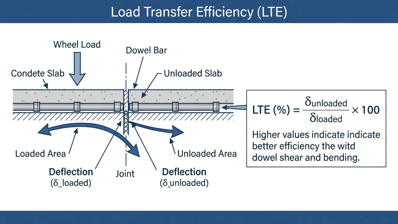
Load Transfer Efficiency (LTE) is a critical structural parameter for jointed plain concrete pavements (JPCP) that quantifies how effectively a load applied to one side of a joint is transferred to the adjacent slab. LTE is evaluated during FWD testing by positioning the loading plate with its edge flush against the joint on the approach slab (the side where traffic first contacts the joint) and placing geophone sensors on both the loaded slab (approach side) and the unloaded slab (leave side) at equal distances from the joint. Typically, sensors are placed at 12 inches (305 mm) on each side of the joint centerline. The FWD applies a load and the deflections on both slabs are recorded simultaneously.

The Load Transfer Efficiency based on deflection (LTEδ) is calculated as:

LTEδ = (D_unloaded / D_loaded) × 100%

Where D_unloaded is the deflection of the slab on the unloaded (leave) side of the joint and D_loaded is the deflection of the slab on the loaded (approach) side of the joint. The LTEδ value theoretically ranges from 0% (no load transfer — the two slabs act independently) to 100% (perfect load transfer — the joint acts as if it were a monolithic slab section). In practice, load transfer efficiencies above 80% are considered excellent for a working joint with well-functioning dowel bars. LTEδ values between 60% and 80% indicate moderate load transfer that may be acceptable for low-volume facilities but should be monitored on high-traffic pavements. LTEδ values below 60% typically indicate joint deterioration — broken or corroded dowel bars, loss of aggregate interlock, or erosion of the subgrade/subbase support beneath the joint — and warrant structural intervention.

The Load Transfer Efficiency based on applied stress or strain (LTEσ) is calculated using a similar ratio but is more difficult to measure in the field, requiring strain gauges or embedded sensors. In practice, LTEδ is the standard metric because it can be measured non-destructively with the FWD sensor array.

The interpretation of LTEδ must consider the joint type. Contraction joints in JPCP typically rely on dowel bars for load transfer, with aggregate interlock providing supplemental transfer through the fractured surface at the bottom of the saw-cut. Construction joints (tied or untied) use tie bars or dowel bars depending on the joint design. Expansion joints use smooth dowel bars designed to allow slab expansion while maintaining vertical load transfer. Longitudinal joints between lanes rely primarily on aggregate interlock at the weakened plane joint or on tie bars for tied longitudinal joints. The expected LTEδ varies by joint type: dowel-bar contraction joints should exhibit LTEδ > 80% after curing; aggregate interlock joints typically exhibit LTEδ of 60 to 80%; and deteriorated or non-functional joints exhibit LTEδ below 40%.

FAA AC 150/5370-11B specifies that LTEδ values below 60% typically indicate joint deterioration requiring further investigation, while D0 values exceeding 0.010 inches (0.25 mm) with low adjacent sensor deflections may indicate voids beneath the slab. The void detection procedure uses the ratio of deflection at the joint corner to the deflection at the slab interior — a high ratio suggests loss of support beneath the slab corner, which can lead to pumping, faulting, and slab cracking.

LTE testing is typically performed at a minimum of 10 test locations per homogeneous pavement section, as defined by the ASTM D6433 (Standard Practice for Pavement Condition Index Surveys) methodology. The FWD test locations should represent the typical joint condition within the section, including joints at slab corners, mid-panel joints, and joints adjacent to the pavement edge. The test results are used to document the structural condition of joints for pavement management systems, identify joints requiring load transfer restoration (dowel bar retrofit), and provide input for rigid pavement overlay design using procedures that account for the existing joint load transfer condition.

Remaining Life Estimation

The back-calculated layer moduli from FWD testing provide the structural basis for estimating the remaining service life of a pavement — the number of years or traffic load repetitions the pavement can carry before reaching terminal serviceability and requiring major rehabilitation. Remaining life estimation requires three components: the current structural capacity (from back-calculated moduli), the expected future traffic loading, and a failure criterion (the terminal pavement condition at which rehabilitation is required).

The Cumulative Damage Factor (CDF) approach, based on Miner’s hypothesis of linear cumulative damage, is the most widely used method for remaining life estimation. The CDF accumulates damage from each traffic load application as a fraction of the allowable number of applications to failure:

CDF = Σ (ni / Ni)

Where ni is the number of applied load repetitions of load level i and Ni is the number of allowable load repetitions of load level i to failure, determined from the appropriate fatigue or rutting transfer function. A CDF of 1.0 indicates that the pavement has consumed its full structural life (100% damage). A CDF of 0.5 indicates that 50% of the structural life has been consumed. The remaining life is:

Remaining Life (%) = (1 - CDF) × 100% Remaining Life (years) = Remaining Life (%) × Design Life (years)

The fatigue transfer function for flexible pavements — relating tensile strain at the bottom of the HMA layer to allowable load repetitions — is one of two primary failure criteria. The Asphalt Institute (AI) fatigue equation (Asphalt Institute MS-1, 9th Edition) is:

Nf = 0.00432 × C × 10^4.84 × (1/εt)^3.291 × (1/E)^0.854

Where Nf is the number of load repetitions to fatigue failure, εt is the maximum tensile strain at the bottom of the HMA layer (from layered elastic analysis using the back-calculated moduli), E is the HMA modulus at the reference temperature, and C = 10^[4.84 × (Vb / (Va + Vb) - 0.69)] where Vb is the effective asphalt content by volume and Va is the air void content.

The Shell fatigue equation uses a similar form:

Nf = C × 10^6 × (1/εt)^n

Where C and n are material constants dependent on the HMA mixture type (typically n = 4.0 to 5.0). For the Shell rutting criterion, the allowable vertical compressive strain at the top of the subgrade is:

εv_allowed = 0.0085 × (Nf/10^6)^(-0.284)

This criterion limits subgrade rutting to prevent structural rutting that propagates upward through the pavement layers, causing surface rutting and serviceability loss.

For the AASHTO 1993 method, remaining life is computed using the concept of structural capacity consumption. The effective structural number (SN_eff) is determined from the back-calculated moduli using the layer coefficient approach:

SN_eff = a1 × D1 + a2 × D2 × m2 + a3 × D3 × m3

Where a1, a2, a3 are the layer coefficients for HMA (a1 = 0.44 per inch typically), base (a2 = 0.14 per inch for granular base), and subbase (a3 = 0.11 per inch for granular subbase), D1, D2, D3 are layer thicknesses, and m2, m3 are drainage coefficients (typically 0.80 to 1.40 depending on drainage quality and saturation exposure). The required structural number (SN_required) for future traffic is determined from the AASHTO performance equation using the design reliability, subgrade modulus, terminal serviceability, and cumulative design ESALs. The reduction in required overlay thickness is proportional to the remaining structural capacity:

SN_overlay = SN_required - SN_eff × RLF

Where RLF is the remaining life factor that accounts for the reduced fatigue life of an existing pavement that has already accumulated damage. RLF varies from approximately 0.5 (when the existing pavement has consumed most of its structural life without showing severe distress) to 1.0 (when the existing pavement is in good structural condition). The overlay thickness (D_ol) is determined as D_ol = SN_overlay / a_ol, where a_ol is the overlay layer coefficient.

The MEPDG/AASHTOWare approach to remaining life uses the back-calculated moduli within the mechanistic-empirical framework. The moduli establish the current structural condition, and the remaining life is computed by: (1) defining the initial condition (current moduli, distress levels, IRI); (2) defining the future traffic loading as axle load spectra; (3) inputting climate data (hourly temperature, precipitation, freeze-thaw cycles); (4) incrementally computing damage accumulation using the mechanistic response model with updated moduli; and (5) predicting the year at which each distress criterion (fatigue cracking, rutting, IRI) reaches the terminal threshold. The remaining life is the shortest time to any distress threshold.

FWD for Overlay Design

FWD deflection data and back-calculated layer moduli are central to overlay thickness design — determining the thickness of new asphalt concrete (AC) or Portland cement concrete (PCC) overlay required to extend the pavement’s service life for a specified future traffic period. The overlay design process uses FWD data to quantify the existing pavement’s structural capacity and then determines the additional thickness needed to carry future traffic.

For flexible pavement overlay design using the AASHTO 1993 method, the process follows these steps:

1. Determine existing pavement structural capacity (SN_eff). The effective structural number is computed from back-calculated layer moduli and existing layer thicknesses using the layer coefficient equation described above. Alternatively, SN_eff can be estimated directly from FWD deflection data using the empirical relationship:

SN_eff = 0.4728 × (D0/0.001)^(-0.4810) × (D0 - D2)^0.0052 × (Mr/1000)^0.2644

Where D0 and D2 are the center and 24-inch sensor deflections in inches, and Mr is the subgrade resilient modulus in psi. This relationship was developed from the AASHO Road Test data and subsequent validation studies.

2. Determine required structural number (SN_required). The SN_required is determined from the AASHTO 1993 flexible pavement performance equation for the design reliability, subgrade modulus, terminal serviceability, and cumulative future ESALs (W18). This is typically solved using the AASHTO nomograph or design equation.

3. Compute overlay structural number requirement. SN_overlay = SN_required - SN_eff × RLF, where RLF accounts for the remaining fatigue life of the existing pavement. The remaining life factor is calculated as:

RLF = exp[-0.436 × (1 - RL)]

Where RL is the remaining life ratio (ratio of remaining life to total design life, from 0.0 to 1.0). A pavement with 100% remaining life has RLF = 1.0, while a pavement at terminal serviceability (0% remaining life) has RLF = 0.54, meaning only 54% of the new overlay’s structural capacity can be credited to the existing pavement.

4. Convert to overlay thickness. D_ol = SN_overlay / a_ol, where a_ol is the layer coefficient for the overlay HMA mixture (typically 0.40 to 0.50 per inch depending on the mix type and quality). Standard HMA overlays use a_ol = 0.44 per inch, while high-modulus overlays may use 0.50 per inch.

5. Apply minimum overlay thickness. AASHTO requires a minimum overlay thickness of 2 inches (50 mm) for structural overlays and 1.5 inches (38 mm) for non-structural overlays. The minimum ensures adequate compaction and bonding between the overlay and existing surface.

For rigid pavement overlay design, the AASHTO 1993 method uses the effective slab thickness (D_eff) determined from FWD back-calculation rather than the structural number. The D_eff is computed from the back-calculated PCC modulus (E_PCC) and the measured deflection using:

D_eff = (P × k / d)^(1/3)

Where P is the FWD load, k is the modulus of subgrade reaction (back-calculated from the subgrade modulus using the relationship k = Mr / 19.4 for typical subgrade conditions), and d is the deflection parameter. The required overlay thickness for rigid pavements is determined by solving the AASHTO rigid pavement performance equation for the slab thickness needed for future traffic (D_required), then computing the overlay thickness as:

D_ol = (D_required^2 - D_eff^2)^0.5 (for unbonded PCC overlays)

Or accounting for partial bonding through composite section analysis for bonded PCC overlays.

The FAA method for airport pavement overlay design using FAARFIELD 2.0 follows a different approach based on layered elastic analysis and cumulative damage. The back-calculated moduli from BAKFAA are input directly into FAARFIELD, which: (1) computes the remaining structural life of the existing pavement under the future traffic mix; (2) determines the required overlay thickness by incrementally adding thickness until the cumulative damage factor (CDF) reaches 1.0 at the end of the design life; and (3) validates the overlay design for the full range of aircraft expected to operate on the pavement, not just the critical design aircraft. FAA AC 150/5320-6G requires a minimum HMA overlay thickness of 3 inches (75 mm) for airport pavements and a minimum PCC overlay thickness of 6 inches (150 mm).

FWD Data Integration with Visual Inspection

The integration of FWD deflection data with visual inspection findings provides the most complete and reliable assessment of pavement condition. Visual inspection (documented through the Pavement Condition Index or PCI per ASTM D6433) identifies surface distress — cracking types and extent, rutting, raveling, patching, faulting, spalling — but provides limited information about the structural condition below the surface. FWD testing provides the structural dimension — layer moduli, load transfer efficiency, and remaining life — but cannot identify specific distress types or functional deficiencies such as poor ride quality or surface texture. The two methods are complementary.

The correlation between PCI and FWD structural parameters provides the bridge between surface condition and structural capacity. A pavement with a high PCI (80-100) but low ISM (below 50 kN/mm) is likely to exhibit rapid deterioration as structural damage accumulates below the surface before appearing as visible distress. Conversely, a pavement with extensive surface cracking but high ISM (above 100 kN/mm) may have adequate structural capacity — the surface distress may be caused by environmental factors (thermal cracking, oxidation) rather than structural loading. In this case, surface treatments (crack sealing, surface seal, thin overlay) may be sufficient without major structural rehabilitation.

The following correlations between visual distress and FWD structural parameters guide integrated pavement evaluation:

Fatigue (alligator) cracking progressing from low to high severity is the most direct surface manifestation of structural fatigue from repeated traffic loading. The extent and severity of alligator cracking should correlate with the cumulative damage factor (CDF) from back-calculated moduli. A pavement with extensive high-severity alligator cracking and CDF approaching 1.0 confirms structural fatigue failure. A pavement with alligator cracking but CDF well below 1.0 suggests that the cracking may be caused by other mechanisms — reflective cracking from underlying stabilized layers, construction deficiencies (segregation, poor compaction), or stripping of the HMA from moisture damage.

Rutting can have two distinct structural causes identifiable from FWD data. Structural rutting — permanent deformation in the subgrade that propagates upward through all pavement layers — is indicated by high vertical compressive strains at the top of the subgrade (εv > 200 microstrain) from layered elastic analysis using back-calculated moduli. Surface rutting — permanent deformation confined to the HMA layer from shear flow at high temperatures — is indicated by low HMA modulus (E_HMA < 200,000 psi at 68°F) without subgrade weakness. The distinction between these rutting mechanisms is critical for selecting the appropriate rehabilitation strategy: structural rutting requires increasing the pavement structural capacity (overlay or reconstruction), while surface rutting can be addressed by milling the existing surface and replacing with a rut-resistant HMA mixture.

Transverse cracking appearing at regular intervals (20 to 40 feet / 6 to 12 m spacing) is typically caused by thermal shrinkage of the HMA layer — a material property issue rather than a structural loading issue. The FWD deflection basin at a transverse crack will show a local increase in D0 and a decrease in LTE across the crack compared with the uncracked pavement. Low LTE across transverse cracks (below 50%) indicates that the crack is working as an uncontrolled joint, reducing the structural continuity of the pavement.

Joint faulting in JPCP — differential vertical displacement at transverse joints — is caused by: (1) erosion of the subgrade/subbase material beneath the approach slab due to water pumping; (2) loss of load transfer efficiency from dowel bar deterioration; and (3) subgrade weakening from moisture accumulation. FWD testing with the joint LTE protocol quantifies the dowel bar condition through LTEδ measurements, and the deflection magnitude at the joint (D0 approach) indicates the structural support condition. High joint deflections (D0 > 0.010 inches at 9,000 lbf) with low LTE (LTEδ < 60%) indicate joint failure requiring load transfer restoration.

The integrated evaluation protocol recommended by the FHWA for project-level structural evaluation specifies: (1) conduct visual PCI survey to identify distress types, severity, extent, and homogeneous pavement sections; (2) perform FWD testing at a minimum of 10 test locations per homogeneous section, with additional tests at distress features (cracks, joints, patched areas); (3) back-calculate layer moduli for each test location and compute section average moduli; (4) overlay PCI data on station-by-station FWD modulus and LTE profiles; (5) identify sections where PCI and FWD data agree (confirming structural diagnosis) and sections where PCI and FWD data disagree (indicating non-structural distress mechanisms or construction anomalies); and (6) develop rehabilitation recommendations based on the integrated assessment.

FWD in Airport Pavement Evaluation (BAKFAA)

Airport pavement evaluation using FWD/HWD testing follows standards and procedures that differ from highway pavement evaluation in several critical aspects. The Heavy Weight Deflectometer (HWD) — a variant of the FWD capable of applying loads from 30,000 to 54,000 lbf (134 to 240 kN) — is the standard equipment for airport pavement testing because aircraft landing gear loads far exceed highway truck loads. FAA AC 150/5370-11B (Use of Nondestructive Testing in the Evaluation of Airport Pavements) specifies the equipment requirements, test procedures, and data analysis protocols for airport FWD/HWD testing.

The standard sensor configuration for airport FWD/HWD testing uses 7 to 9 geophone sensors at offsets of 0, 12, 24, 36, 48, 60, and 72 inches (0, 305, 610, 914, 1,219, 1,524, and 1,829 mm) from the load center, matching the highway configuration but with sensors capable of measuring deflections up to 0.080 inches (2.0 mm) at the center sensor. The drop sequence requires: 4 seating drops to ensure proper plate contact, followed by 3 recording drops at each of 2 to 3 load levels (typically 12, 24, and 36 kip / 53, 107, and 160 kN). The test spacing on runways is 100 to 400 feet (30 to 120 m) in the wheel paths, with additional tests at centerline and edge locations. On aprons and taxiways, the testing interval is 50 to 100 feet (15 to 30 m) in a grid pattern to provide full coverage.

BAKFAA is the FAA-authorized back-calculation software for airport pavements (FAA AC 150/5370-11B, Chapter 7). BAKFAA uses the LEAF (Layered Elastic Analysis, FAA) forward engine, developed specifically for airport pavement analysis with the following capabilities: layered elastic analysis for up to 5 pavement layers; support for multi-wheel aircraft landing gear configurations (critical for aircraft such as the B-747 with 4 main gear struts, the B-777 with 6 main gear wheels per strut, and the A-380 with 20 main gear wheels); handling of thick PCC slabs (12 to 24 inches / 300 to 600 mm) typical of airport runways; and processing of HWD load data at the high levels required for airport pavements. BAKFAA supports both flexible and rigid pavement analysis — an essential capability for airports that typically have PCC runways and flexible taxiways and aprons.

BAKFAA outputs are directly integrated with FAARFIELD 2.0 (the FAA’s pavement design software) for airport pavement evaluation. The FAARFIELD evaluation process is: (1) back-calculate layer moduli using BAKFAA; (2) input the moduli into FAARFIELD as existing pavement properties; (3) define the aircraft traffic mix (aircraft types, annual departures, and gross weights); (4) FAARFIELD computes the Cumulative Damage Factor (CDF) for each aircraft in the traffic mix, using layered elastic analysis for flexible pavements and 3D finite element analysis (NIKE3D) for rigid pavements; (5) the critical aircraft is identified as the aircraft producing the maximum CDF; and (6) the remaining structural life is estimated by determining the number of years before CDF reaches 1.0.

The ICAO ACR-PCR system (effective November 28, 2024 per ICAO Amendment 15) requires airport pavement bearing strength to be reported using the Pavement Classification Rating (PCR) format. The PCR is determined through the Technical Evaluation method using FWD/HWD data. The 8-step PCR evaluation process is: (1) collect pavement data (FWD deflections, layer thicknesses from cores or GPR, material types); (2) back-calculate layer moduli using BAKFAA; (3) define the aircraft traffic mix (aircraft types, annual departures, gross weights, tire pressures); (4) compute ACR (Aircraft Classification Rating) for each aircraft type in the mix; (5) compute CDF for the existing traffic mix using FAARFIELD; (6) identify the critical aircraft (the aircraft producing the maximum CDF); (7) adjust the critical aircraft weight to achieve CDF = 1.0; and (8) compute the PCR from the adjusted critical aircraft weight. The PCR is reported as a five-part code: PCR [value] / [Pavement Type R or F] / [Subgrade Strength A, B, C, or D] / [Tire Pressure W, X, Y, or Z] / [Evaluation Method T for Technical] .

The ICAO subgrade strength categories for PCR are determined from the back-calculated subgrade modulus (E) according to: Category A (High): E ≥ 150 MPa (21,750 psi); Category B (Medium): 60 < E ≤ 150 MPa (8,700 to 21,750 psi); Category C (Low): 20 < E ≤ 60 MPa (2,900 to 8,700 psi); Category D (Ultra Low): E ≤ 20 MPa (2,900 psi). The subgrade modulus obtained from FWD back-calculation is therefore a direct input to the ICAO bearing strength reporting system, making its accuracy essential for international airport pavement classification compliance.

The FAA recommends FWD/HWD testing frequency for airport pavements of every 3 to 5 years for major hub runways, every 5 to 7 years for general aviation runways, and before any overlay design (single event required). Each evaluation should include a structural evaluation report documenting: deflection basin parameters (D0, AREA, ISM); back-calculated moduli for each pavement section; LTE values for jointed PCC pavements; remaining life estimates; overlay thickness recommendations if required; and the PCR assignment per ICAO Annex 14. The annual FAA Airport Pavement Management System (APMS) requires structural data from FWD testing to be integrated with PCI survey data for network-level pavement condition tracking and capital improvement planning for AIP- and PFC-funded projects.

The integration of FWD deflection data analysis and back-calculation with visual inspection, remaining life estimation, and structural design provides a complete pavement management framework. The quantitative layer moduli from back-calculation explain the root causes of observed surface distress — a weak subgrade causes structural rutting, a deteriorated base causes fatigue cracking from below, and temperature-softened HMA causes surface rutting. Without the structural dimension from FWD testing, pavement evaluation is limited to describing what can be seen on the surface. The back-calculation process transforms the FWD deflection basin — a simple set of surface measurements — into a complete picture of pavement structural health, enabling engineers to design targeted, cost-effective rehabilitation strategies that address the actual structural deficiencies rather than treating surface symptoms.