What is GPS accuracy?
GPS Accuracy for Infrastructure Survey and Inspection
Definition: What is GPS accuracy?
GPS accuracy is the quantifiable measure of how closely a GNSS (Global Navigation Satellite System) receiver-computed position matches the true physical coordinates on the Earth’s surface. It is expressed as a statistical probability that a position fix falls within a specified distance from the true location, for example, “1.5 meters horizontal accuracy at 95% confidence” means that 95 out of 100 position fixes will fall within a 1.5-meter radius of the true point. GPS accuracy is fundamentally distinct from precision (the repeatability of measurements) and resolution (the smallest unit a receiver can detect), though all three terms are frequently confused in practice.
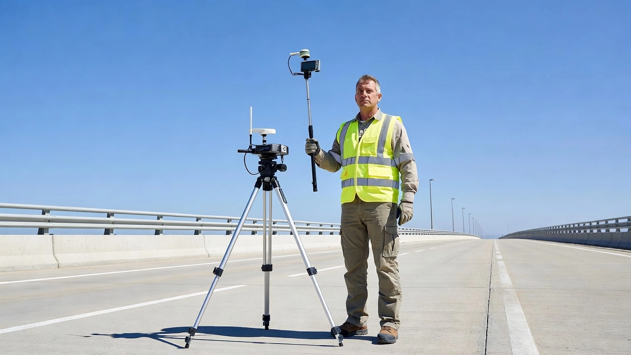
In infrastructure survey and inspection, GPS accuracy dictates which positioning method is viable for a given task. A coarse asset inventory on a highway may tolerate 3-meter errors, whereas photogrammetric ground control point establishment for crack-width measurement requires sub-centimeter accuracy. The achievable accuracy depends on the GNSS technology employed, autonomous GPS, Differential GPS (DGPS), Satellite-Based Augmentation Systems (SBAS), Real-Time Kinematic (RTK), Post-Processed Kinematic (PPK), or static survey, and the environmental conditions under which measurements are taken.
The International Civil Aviation Organization (ICAO) Annex 10, Volume I (Aeronautical Telecommunications) defines GPS accuracy standards for aviation navigation, specifying accuracy requirements for different phases of flight: en-route navigation requires ±3.7 km (2 NM) accuracy 95% of the time, while Category I precision approaches require ±16 m horizontal and ±4 m vertical. For surveying and inspection, standards from the International Organization for Standardization (ISO 17123-8), which specifies field procedures for testing GNSS field measurement systems, and national surveying authorities (e.g., FGDC in the U.S., Ordnance Survey in the UK) govern accuracy reporting. The U.S. Federal Radionavigation Plan, published jointly by the Department of Defense and the Department of Transportation, is the authoritative source for GPS accuracy specifications, stating that the Standard Positioning Service (SPS) provides horizontal accuracy of ≤9 m (95%) and vertical accuracy of ≤15 m (95%).
A GPS position is never perfectly accurate, rather, it carries an error budget, a combination of satellite, atmospheric, receiver, and environmental errors that degrade the solution. Understanding this error budget is the prerequisite for selecting the appropriate positioning method for any infrastructure inspection task.
GPS Error Sources
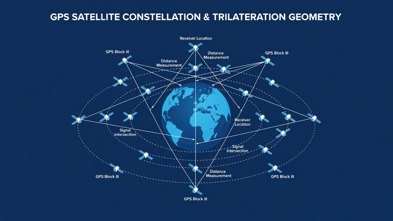
The total error in a standalone GPS position fix is the root-sum-square (RSS) combination of several independent error sources, each with characteristic magnitude and behavior. These errors are classified into three categories: satellite-dependent errors (clock and ephemeris), signal propagation errors (ionosphere and troposphere), and receiver-dependent errors (multipath and receiver noise).
Satellite Clock Errors
Each GPS satellite carries multiple atomic clocks, typically two cesium and two rubidium atomic frequency standards, that are monitored and adjusted by the control segment’s master control station at Schriever Air Force Base in Colorado. Despite their precision (cesium clocks are accurate to 1 part in 10¹³), residual clock errors remain. A clock offset of just 10 nanoseconds translates to a 3-meter range error because the GNSS ranging measurement multiplies signal travel time by the speed of light (299,792,458 m/s). The control segment estimates clock corrections using the L-band navigation message uploads, broadcasting clock correction parameters (af0, af1, af2) in subframe 1 of the GPS navigation message. Residual errors of 1 to 2 meters persist in the broadcast navigation message. The effect is common to all receivers viewing the same satellite, making it highly correlated, which is why differential techniques cancel this error almost completely.
Orbit (Ephemeris) Errors
The broadcast ephemeris, the set of Keplerian orbital parameters transmitted by each satellite in subframes 2 and 3 of the GPS navigation message, describes the satellite’s position at any given time. The control segment computes these parameters from tracking data collected by 16 monitor stations distributed globally, but residual orbit errors of 0.5 to 2.5 meters remain. The U.S. Space Force’s 2nd Space Operations Squadron publishes precise ephemeris data (accuracy <5 cm) through the International GNSS Service (IGS), but this is only available post-mission (for post-processing) or via real-time services like the NASA GDGPS (Global Differential GPS) system. Ephemeris errors manifest as an along-track, cross-track, and radial displacement of the satellite position, which propagates directly into the user’s position solution with an amplification factor of 0.5 to 1.5 depending on the component.
Ionospheric Delay
The ionosphere, the ionized layer of the atmosphere from approximately 50 to 1,000 km altitude, is the largest single source of GPS error for single-frequency receivers. Charged particles in the ionosphere slow the GPS radio signals (group delay for the code and phase advance for the carrier), introducing path delays that vary with solar activity (the 11-year solar cycle causes delays to vary by a factor of 5 between solar minimum and maximum), time of day (delays peak in local afternoon when solar radiation is strongest, with a diurnal variation of 2-10 meters), elevation angle (signals from low-elevation satellites traverse more ionosphere, the slant delay at 5° elevation is approximately three times the zenith delay), and geographic location (equatorial regions within ±20° latitude experience the highest ionospheric variability and often exhibit plasma bubbles that cause scintillation, while polar regions experience particle precipitation effects).
Typical zenith ionospheric delay is 2 to 5 meters, but can reach 50 meters during periods of high solar activity and at low elevation angles. Dual-frequency receivers can virtually eliminate ionospheric error by comparing the L1 (1575.42 MHz) and L2 (1227.60 MHz) signal delays, as the ionosphere is a dispersive medium. Single-frequency receivers rely on the Klobuchar model (parameters broadcast in the GPS navigation message as eight coefficients), which corrects approximately 50% of the delay under nominal conditions. The newer NeQuick-G model adopted by Galileo provides improved performance, correcting approximately 70% of the delay.
Tropospheric Delay
The troposphere, the lowest atmospheric layer from the surface to approximately 12 km altitude, introduces a non-dispersive delay that affects all GNSS frequencies equally. Unlike the ionosphere, the troposphere cannot be corrected by dual-frequency measurements because the delay is frequency-independent. Tropospheric delay consists of a dry component (about 90% of the total, driven by atmospheric pressure and temperature, approximately 2.3 meters at zenith under standard conditions) and a wet component (about 10%, driven by water vapor content, highly variable, from a few millimeters to 30-40 cm at zenith in humid conditions).
Typical zenith tropospheric delay is 2.0 to 2.5 meters, varying with weather conditions. Standard tropospheric models (e.g., Saastamoinen, Hopfield, UNB3, GPT2w) correct 80 to 90% of the delay, leaving 0.2 to 0.5 meters of residual error. In differential GNSS over short baselines (under 10 km), tropospheric errors are largely common to both base and rover and cancel effectively. Beyond 50 km, tropospheric decorrelation becomes significant, with residual errors increasing at approximately 0.1-0.2 mm per km of baseline.
Multipath Error
Multipath occurs when the GNSS signal arrives at the antenna via two or more paths, the direct line-of-sight path plus one or more reflected paths from nearby surfaces such as buildings, vehicles, water bodies, terrain, or the ground itself. The reflected signal has a longer path length and may arrive with opposite phase, causing destructive interference that corrupts the correlation peak in the receiver’s delay-lock loop (DLL) and phase-lock loop (PLL). Typical code multipath errors range from 0.5 to 5 meters, while carrier-phase multipath errors are smaller (1 to 5 cm) but still significant for high-precision work. Mitigation techniques include choke-ring antennas (concentric rings that suppress ground-reflected signals by up to 20 dB), correlation techniques (narrow correlator spacing reduces multipath sensitivity by a factor of 2-5), and antenna placement (minimum 5 meters away from reflective surfaces).
Receiver Noise
Receiver noise encompasses thermal noise in the RF front end, quantization noise in the analog-to-digital converter (ADC), and oscillator phase noise. Typical code measurement noise for a modern receiver is 0.1 to 0.5 meters, while carrier-phase noise is 1 to 5 millimeters. Receiver noise is random and uncorrelated between receivers, it cannot be reduced by differential correction but can be lowered by using higher-quality receivers (geodetic-grade versus consumer-grade), longer integration times, and improved signal processing algorithms.
| Error Source | Typical Magnitude (Standalone) | Mitigation |
|---|---|---|
| Satellite Clock | 1–2 m | Differential correction, precise clock products |
| Orbit (Ephemeris) | 0.5–2.5 m | Differential correction, precise ephemeris |
| Ionosphere (single-frequency) | 2–50 m | Dual-frequency, SBAS, Klobuchar model |
| Troposphere | 0.2–0.5 m residual | Models, differential over short baselines |
| Multipath (code) | 0.5–5 m | Antenna design, site selection |
| Receiver Noise | 0.1–0.5 m | High-quality receiver, signal processing |
Autonomous GPS Accuracy
Autonomous (standalone) GPS accuracy refers to the positioning performance of a single GNSS receiver operating without any external corrections or augmentation. The receiver uses the broadcast navigation message, satellite ephemeris, clock corrections, and ionospheric model parameters, to compute its position from pseudorange measurements only. The GPS Standard Positioning Service (SPS) Performance Standard, published by the U.S. Department of Defense, defines the committed performance level.
Under open-sky conditions with good satellite geometry (HDOP < 2), a modern civilian GPS receiver achieves horizontal accuracy of 3 to 5 meters (95% confidence) and vertical accuracy of 5 to 8 meters (95% confidence) . The user equivalent range error (UERE) budget for autonomous GPS is approximately 2.5 to 3.0 meters RMS, composed of satellite clock (0.5 m), ephemeris (0.4 m), ionosphere (1.5 m for single-frequency), troposphere (0.4 m), multipath (0.5 m), and receiver noise (0.3 m).
The removal of Selective Availability (SA) on May 2, 2000, at 04:00 UTC by U.S. Presidential directive improved standalone GPS accuracy from approximately 100 meters to the current 3-to-5-meter level. SA was the intentional degradation of the civilian GPS signal by dithering the satellite clock. The U.S. government has committed to not reintroducing SA, as stated in the 2010 National Space Policy.
Autonomous GPS is suitable for consumer navigation (smartphones, vehicle navigation), coarse asset tracking where meter-level position is adequate, and time synchronization (GPS time is accurate to within 50 nanoseconds of UTC). For infrastructure inspection, autonomous GPS is generally insufficient for tasks requiring accurate defect geolocation, photogrammetry ground control, or precise measurement, a 5-meter position error can place a pavement crack on the wrong lane of a highway or misidentify the structural element containing a defect.
Differential GPS (DGPS)
Differential GPS (DGPS) is a technique that uses one or more reference stations at known, surveyed locations to compute corrections that are broadcast to rover receivers in the area. The fundamental principle is that nearby receivers experience nearly identical common-mode errors, satellite clock errors (100% correlated), ephemeris errors (highly correlated within 100 km), and atmospheric delays (correlated with baseline length), so subtracting the reference station’s error from the rover’s measurement cancels these shared components.
DGPS correction data is transmitted in standardized formats such as RTCM SC-104 (Radio Technical Commission for Maritime Services, now RTCM 10403.x standard) over VHF radio, UHF radio, satellite, or cellular links. The effective range of a DGPS reference station is typically 100 to 500 km, with correction accuracy degrading as the rover moves farther from the reference due to spatial decorrelation of atmospheric errors.
Achievable accuracy: DGPS typically provides 1 to 3 meters horizontal accuracy (95% confidence) , depending on the quality of the reference station, the distance from it, and local multipath conditions. The International Association of Marine Aids to Navigation and Lighthouse Authorities (IALA) operates a network of maritime DGPS reference stations broadcasting corrections at 283.5-325 kHz (the marine radiobeacon band) for harbor navigation, achieving 2-5 meter accuracy up to 500 km offshore.
DGPS is implemented in three principal forms: Local Area DGPS (LADGPS) using a single reference station broadcasting corrections to local users with a typical range of 50-200 km, Wide Area DGPS (WADGPS) deploying a network of reference stations that models errors over a large region (the architectural foundation of SBAS), and Maritime DGPS following IALA standards using coastal reference stations. For infrastructure inspection, DGPS is appropriate for coarse asset localization, identifying which bridge girder, which section of pavement, or which utility pole has a defect, but is not suitable for applications requiring precise measurements such as crack-width quantification, settlement monitoring, or photogrammetric control.
SBAS (WAAS, EGNOS, MSAS, GAGAN)
Satellite-Based Augmentation Systems (SBAS) are regional augmentation networks that improve GPS accuracy, integrity, continuity, and availability by broadcasting correction messages via geostationary satellites. SBAS is the satellite-based evolution of DGPS, offering wide-area coverage without requiring the user to deploy a local reference station. ICAO’s Annex 10, Volume I defines the standards for SBAS, specifying that SBAS must support aircraft approaches down to LPV (Localizer Performance with Vertical guidance) minima with decision heights as low as 200 feet.
The principal SBAS systems operating worldwide are:
| System | Coverage Area | Operator | Operational Since | Geostationary Satellites |
|---|---|---|---|---|
| WAAS | North America (USA, Canada, Mexico) | FAA (U.S. FAA) | 2003 | Inmarsat 4-F3, SES-15 |
| EGNOS | Europe | ESA/EU | 2009 | Inmarsat 4-F2, Astra 5B |
| MSAS | Japan and Asia-Pacific | JCAB | 2007 | MTSAT-1R, MTSAT-2 |
| GAGAN | India | ISRO/AAI | 2013 | GSAT-8, GSAT-10 |
| SDCM | Russia | Roscosmos | 2016 | Luch-5A, Luch-5B |
| BDSBAS | China | CNSA | 2020 (under dev.) | BeiDou satellites |
| KASS | South Korea | KARI | 2023 | KT SAT satellite |
SBAS works through a network of reference stations (WRS for WAAS, RIMS for EGNOS) distributed across the coverage area, WAAS has 38 reference stations in the United States and another 20 in Canada and Mexico, while EGNOS has 40 RIMS stations across Europe. These stations continuously monitor GPS signals and relay data to master control stations that compute: ionospheric corrections (grid-based estimates of vertical ionospheric delay at predefined ionospheric pierce points, WAAS uses a 5°×5° grid), satellite orbit and clock corrections (fast corrections applied every 2-6 seconds and long-term corrections applied every 60-120 seconds), and integrity bounds (confidence bounds that guarantee error limits with 10⁻⁷ integrity risk per approach).
The corrections are uplinked to geostationary satellites (Inmarsat 4-F3 at 133°W for WAAS, Inmarsat 4-F2 at 25°E for EGNOS), which broadcast on the GPS L1 frequency (1575.42 MHz) using a unique PRN code. SBAS-capable receivers apply these corrections in real time using the MOPS (Minimum Operational Performance Standards) algorithm defined by RTCA DO-229.
Achievable accuracy: SBAS typically provides horizontal accuracy of 1 to 2 meters (95% confidence) and vertical accuracy of 2 to 4 meters (95% confidence) across the coverage area. WAAS achieved an average horizontal accuracy of 0.5 to 1.0 meters in recent FAA performance assessments, with a worst-case of 1.2 meters across the CONUS service area. This performance enables LPV approaches to minima as low as 200 feet decision height, equivalent to Category I ILS. EGNOS provides similar performance across Europe, with over 77 million flight hours cumulated in safety-of-life service since 2011.
For infrastructure inspection, SBAS is suitable for visual inspection geotagging, associating a photo or observation with a location accurate enough to identify the correct structural element (e.g., which bridge span, which 10-meter section of pavement). It does not provide the centimeter-level accuracy required for photogrammetric ground control or precision defect measurement.
Real-Time Kinematic (RTK) GPS
Real-Time Kinematic (RTK) is the highest-performance real-time GNSS positioning technique, delivering centimeter-level accuracy (1 to 3 cm horizontal, 2 to 5 cm vertical) by using carrier-phase measurements combined with differential corrections from a nearby base station. RTK is the standard positioning method for surveying, machine control, precision agriculture, and high-accuracy drone mapping. The technique was first developed in the 1980s by surveying instrument manufacturers and has since been refined through multi-frequency, multi-constellation receivers.

How RTK Works
RTK uses the carrier wave of the GNSS signal rather than the code modulation. The L1 carrier wavelength is approximately 19 cm, compared to the C/A code chip length of approximately 293 meters. By measuring the fractional carrier phase to millimeter-level precision and resolving the integer ambiguity (the unknown number of full carrier cycles between satellite and receiver), RTK achieves measurement resolution of a few millimeters. The carrier-phase observation equation is: Φ = ρ + c(dt - dT) + I + T + λN + ε, where Φ is the carrier-phase measurement, ρ is the geometric range, dt and dT are the satellite and receiver clock errors, I and T are the ionospheric and tropospheric delays, λN is the integer ambiguity term (λ = wavelength, N = integer number of cycles), and ε is measurement noise.
The RTK system architecture consists of three components: (1) a base station, a GNSS receiver at a precisely surveyed known location (coordinates established via static survey or known to centimeter-level from a control network) that tracks all visible satellites and computes corrections, (2) a communication link, transmits corrections from base to rover in real time via UHF radio (typically 400-470 MHz with range of 5-15 km), 4G/5G cellular, WiFi, or NTRIP (Networked Transport of RTCM via Internet Protocol) over the internet, and (3) a rover receiver, applies base station corrections to its own carrier-phase measurements using double-difference processing, resolving integer ambiguities and computing a precise position in real time.
Ambiguity resolution, the process of determining the correct integer number of carrier cycles, is the critical step in RTK. Modern multi-frequency, multi-constellation receivers achieve fixed ambiguity resolution in 2-10 seconds under good conditions using techniques such as LAMBDA (Least-squares AMBiguity Decorrelation Adjustment), TCAR (Three-Carrier Ambiguity Resolution), or MLAMBDA. The RTK fix quality is indicated by three states: Fixed solution (all ambiguities resolved to integers, accuracy 1-3 cm), Float solution (ambiguities estimated as real numbers without integer resolution, accuracy 20-50 cm), and Single (autonomous) solution (no differential corrections applied, accuracy 3-5 m).
Modern RTK systems use multi-constellation GPS + GLONASS + Galileo + BeiDou for improved satellite availability (typically 30+ visible satellites versus 8-12 for GPS alone), and multi-frequency (L1/L2/L5) for faster ambiguity resolution and improved reliability in challenging environments. Network RTK (also called RTK Network or NRTK) extends RTK coverage by using a regional network of reference stations (typically 50-100 km spacing) that models atmospheric errors across the network area, the rover receives corrections specific to its approximate location.
RTK Limitations
RTK accuracy degrades with distance from the base station at approximately 1 ppm (1 mm per km of baseline) horizontally and 2 ppm vertically due to spatial decorrelation of atmospheric errors. Beyond 10 to 20 km, residual errors become significant, requiring network RTK or PPP-RTK techniques. The communication link between base and rover must maintain a data rate of 4800-9600 bps (RTCM 3.x format) with latency under 2 seconds, loss of the correction stream causes the rover to fall back to float or single solutions within 30-60 seconds. Carrier-phase measurements are more susceptible to cycle slips from multipath interference, and ambiguity resolution requires a brief initialization period in stationary or low-dynamics conditions.
For infrastructure inspection, RTK is essential for ground control point (GCP) establishment for drone photogrammetry, precision defect geolocation where sub-decimeter accuracy is required, machine control for construction and rehabilitation projects, and bridge deflection monitoring with centimeter precision.
Post-Processed Kinematic (PPK)
Post-Processed Kinematic (PPK) is an alternative to RTK that achieves the same centimeter-level accuracy (1 to 3 cm) but processes the GNSS data after the mission rather than in real time. Instead of requiring a continuous communication link between base and rover, PPK records raw GNSS observation data on both the base station and the rover, typically in RINEX (Receiver Independent Exchange Format) format, and these are combined in software after data collection.
How PPK Works
During the mission, both the base station and the rover record raw GNSS data simultaneously, carrier-phase measurements, pseudoranges, satellite ephemeris, and signal-to-noise ratios at a logging rate of 1-10 Hz. After the mission, post-processing software (e.g., RTKLIB, open-source, Trimble Business Center, DJI Terra, POSPac UAV, NovAtel Waypoint) combines the base and rover observations using double-difference carrier-phase processing to resolve integer ambiguities and compute precise positions for each rover epoch. The processing software can apply forward and backward filtering (Kalman smoothing) that improves accuracy by 10-20% compared to forward-only processing.
PPK offers several advantages over RTK: no communication link required, the rover does not need real-time corrections from the base, making PPK ideal for remote areas, urban canyons, and UAV operations where radio links are unreliable, post-processing flexibility, data can be re-processed with improved ephemeris (IGS precise orbit and clock products with <2.5 cm accuracy), refined error models, and manual cycle-slip repair, higher accuracy potential, PPK achieves accuracy marginally better than RTK because processing software applies forward/backward smoothing and uses precise satellite products rather than broadcast ephemeris, and reduced receiver burden, the PPK rover does not need to resolve ambiguities in real time, reducing computational requirements and power consumption by 15-25%.
PPK is particularly advantageous for UAV-based infrastructure inspection. Drones operating at distances from the base station that exceed reliable radio range, or in terrain that blocks radio signals (valleys, structures), benefit from PPK’s independence from real-time links. The DJI Mavic 3 Enterprise, Matrice 300 RTK, and Matrice 4E all support PPK workflows by recording raw GNSS observations onboard (typically at 1-2 Hz logging rate).
| Factor | RTK | PPK |
|---|---|---|
| Accuracy | 1–3 cm | 1–3 cm |
| Real-time position | Yes | No (post-processed only) |
| Communication link | Required (radio, NTRIP) | Not required |
| Post-processing time | None | 10-60 minutes per mission |
| Suitability for UAV | Good (if radio link reliable) | Excellent (remote/obstructed areas) |
| Data storage | Minimal (position output) | Raw data storage (RINEX: 5-15 MB per hour) |
| Cycle slip handling | Real-time algorithms | Forward/backward smoothing in software |
| Precise ephemeris use | No (broadcast only) | Yes (IGS final products available 2 weeks later) |
Static Survey
Static survey is the highest-accuracy GNSS positioning technique, achieving sub-centimeter horizontal accuracy (typically 2.5 mm + 1 ppm horizontally, 5 mm + 1 ppm vertically) through extended data collection periods and post-processing. Static surveys are used to establish control networks, monument positions, and reference points that serve as the foundation for all lower-accuracy measurements in a project area.
How Static Survey Works
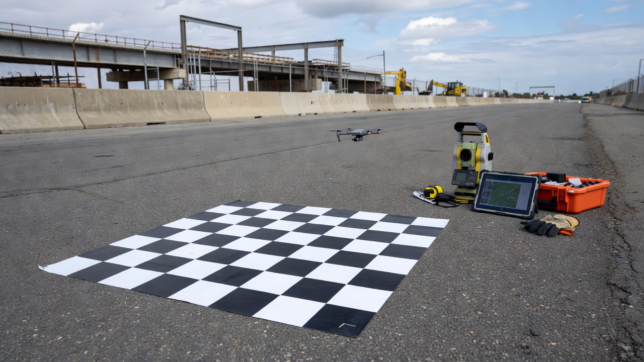
Static survey involves deploying two or more GNSS receivers at fixed locations for an extended period, typically 40 minutes to several hours or even multiple days (24-hour sessions for ultra-high accuracy). The receivers track all visible satellites continuously, recording raw carrier-phase and pseudorange observations at a high rate (1 Hz to 50 Hz). All receivers collect data simultaneously, and post-processing software computes the baseline vectors between each pair of receivers using double-difference carrier-phase processing with full ambiguity resolution. The long observation period allows the receiver to collect data through changing satellite geometry, changing multipath patterns, and varying atmospheric conditions.
Key characteristics include long occupation time (40+ minutes for short baselines under 10 km, 2+ hours for 50 km baselines, and 4+ hours or overnight for baselines over 100 km), baseline length capability from 50 km to 1,000 km or more with accuracy degrading linearly with distance (the “ppm” term: each kilometer of baseline adds approximately 1 mm of error horizontally and 2 mm vertically), and multi-station adjustment in which observations from multiple receivers and multiple sessions are combined in a least-squares network adjustment that computes optimal coordinates for all stations with statistical quality indicators.
The observation time equation for static surveying follows the rule of thumb: T (minutes) = 30 + 3 × baseline length (km) / number of visible satellites, for a 50 km baseline with 12 visible satellites, approximately 42 minutes minimum.
Static Survey Accuracy Specifications
Survey-grade receivers achieve the following published accuracies: horizontal, 3 mm + 0.5 ppm RMS (Leica GS18, Trimble R12i), vertical, 5 mm + 0.5 ppm RMS. The ppm component means that for a 10 km baseline, horizontal accuracy is 3 mm + 5 mm = 8 mm RMS, and for a 200 km baseline, 3 mm + 100 mm = 103 mm (10.3 cm) RMS. Static survey is the recommended technique for National Geodetic Survey (NGS) control networks in the United States, where order A (0.5 mm + 0.01 ppm) to order C (10 mm + 1 ppm) accuracy classifications apply.
In infrastructure inspection, static survey is used to establish ground control points (GCPs) for photogrammetric projects, monitor structural deformation over time (bridge settlement, bridge deflection, retaining wall movement, pavement settlement), calibrate and validate lower-accuracy positioning methods (RTK, PPK, DGPS), and provide reference coordinates for base stations used in RTK/PPK operations.
Dilution of Precision (GDOP, PDOP, HDOP, VDOP)
Dilution of Precision (DOP) is a dimensionless metric that describes how satellite geometry affects the quality of a GPS position solution. DOP acts as a multiplier on the measurement error: a receiver with 3-meter pseudorange errors and a PDOP of 2 will have a 3D position error of approximately 6 meters (3 m × 2.0 = 6.0 m RMS). Lower DOP values indicate better satellite geometry and smaller error propagation. The concept was first formalized in the 1980s as part of the GPS System Specification (SS-GPS-200).
Types of DOP
| DOP Type | Components | Application |
|---|---|---|
| GDOP (Geometric DOP) | Position (3D) + Time | Overall system performance assessment |
| PDOP (Position DOP) | 3D position (lat, lon, alt) | 3D positioning quality |
| HDOP (Horizontal DOP) | Latitude and longitude | Horizontal positioning quality |
| VDOP (Vertical DOP) | Altitude only | Vertical positioning quality |
| TDOP (Time DOP) | Receiver clock error | Timing quality |
DOP Values and Interpretation
| DOP Value | Rating | Interpretation |
|---|---|---|
| 1 | Ideal | Optimal satellite geometry |
| 2–3 | Excellent | Suitable for high-precision surveying and RTK |
| 4–5 | Good | Suitable for general navigation and DGPS |
| 6–7 | Moderate | Acceptable but accuracy degraded |
| 8–10 | Fair | Marginal quality |
| >10 | Poor | Very poor geometry, position unreliable |
How DOP Is Computed
DOP is derived from the receiver-to-satellite geometry matrix (H matrix), which contains the direction cosines from the receiver to each visible satellite. The covariance matrix Q = (HᵀH)⁻¹ diagonal elements give: GDOP = √(Q₁₁ + Q₂₂ + Q₃₃ + Q₄₄), PDOP = √(Q₁₁ + Q₂₂ + Q₃₃), HDOP = √(Q₁₁ + Q₂₂), and VDOP = √(Q₃₃). The matrix H has dimensions n×4 for n visible satellites, with each row containing the direction cosines and a 1 for the clock offset term.
For infrastructure inspection and surveying, operators monitor DOP values in real time: HDOP < 2 is typically required for RTK and PPK operations, PDOP < 3 is recommended for static surveys and control point establishment, and VDOP < 3 is important for applications requiring good vertical accuracy (e.g., bridge clearance assessment, settlement monitoring). DOP is improved by using multi-constellation receivers (GPS + GLONASS + Galileo + BeiDou provides 30+ visible satellites, reducing PDOP by 40-60% compared to GPS alone), setting elevation masks (typically 10° to 15° to remove low-elevation satellites), and scheduling surveys to avoid periods of weak geometry.
HDOP specifically addresses the horizontal component, in urban canyons where building obstructions limit satellites to a narrow sky corridor, HDOP can exceed 3-4. VDOP is consistently 1.5 to 2 times higher than HDOP because satellite geometry is inherently weaker in the vertical dimension, satellites are only visible above the horizon, resulting in asymmetrical geometry. This explains why GPS vertical accuracy is generally 1.5 to 2 times worse than horizontal accuracy. PDOP combines horizontal and vertical components and is the standard metric for survey work acceptance, with most survey-grade receivers configured to reject measurements when PDOP exceeds user-defined thresholds (commonly 4-6). GDOP includes the time component and is typically 5-10% higher than PDOP.
Selecting GPS Accuracy for Infrastructure Inspection Tasks
Different infrastructure inspection tasks require different GPS accuracy levels. Selecting the appropriate positioning method requires understanding the accuracy requirement (absolute vs. relative), the environment (open sky vs. obstructed), the equipment available, and the cost/time budget.
| Inspection Task | Required Accuracy | Recommended GPS Method | Rationale |
|---|---|---|---|
| Coarse asset inventory | 1–5 m | DGPS, SBAS | Adequate for identifying which structure/segment |
| Visual inspection geotagging | 1–3 m | WAAS/SBAS, DGPS | Photo location adequate for retrieval |
| Pavement crack mapping (lane-level) | 0.3–1 m | DGPS, precise code-based | Sufficient for lane-level defect location |
| Photogrammetry ground control | 1–3 cm | RTK, PPK, Static | Required for ortho-rectification and scaling |
| Crack width measurement (drone-based) | 1–3 cm | RTK, PPK | Absolute positioning for precise defect dimensions |
| Bridge deflection monitoring | 0.5–2 cm | Static survey (epoch-to-epoch) | Sub-centimeter repeatability required |
| Settlement monitoring | 0.2–1 cm | Static survey | Highest accuracy for vertical change detection |
| Machine control (construction) | 2–5 cm | RTK | Real-time centimeter guidance for earthmoving |
| UAV LiDAR georeferencing | 3–10 cm | PPK, RTK | Direct georeferencing of point cloud |
Absolute vs. Relative Accuracy in Inspection
A critical distinction in inspection workflows is between absolute accuracy (how close measurements are to true global coordinates in WGS84, ITRF, or a local datum) and relative accuracy (how well points within the same dataset relate to each other). RTK, PPK, and static survey provide high absolute accuracy (1-3 cm globally referenced), while autonomous GPS and DGPS provide lower absolute accuracy. For some inspection tasks, like measuring crack width in a single orthophoto, relative accuracy may be sufficient even if absolute accuracy is poor. However, for multi-epoch monitoring (comparing crack widths over months or years), both relative and absolute accuracy matter because the alignment between epochs depends on absolute coordinates.
Environmental Considerations
GPS accuracy degrades differently in different environments. Under open sky (highways, bridges over water, exposed infrastructure), all methods work well with RTK baselines extending up to 30 km. In urban canyons (city streets, tunnels, under-bridge areas), GNSS signals are blocked or severely degraded, RTK initialization becomes difficult, DOP values rise above 5, and multipath is severe. Alternative positioning methods (total station, SLAM-based LiDAR, or visual odometry) may be needed. Under tree canopy (roads in wooded areas), code-based methods degrade by 30-50%, and carrier-phase methods may experience frequent cycle slips, longer observation times (2-4× normal) are required. Near large structures (bridges, buildings), multipath from reflective surfaces degrades accuracy, antenna placement at least 1 meter away from surfaces is critical.
Choosing Between RTK and PPK for UAV Inspection
For drone-based infrastructure inspection, the choice between RTK and PPK depends on the communication environment (if the drone maintains reliable radio link to the base station throughout flight, RTK provides real-time centimeter positioning with immediate feedback), operational range (beyond 5-10 km from the base station, radio links degrade and PPK becomes preferable, with ranges exceeding 50 km possible using base station-logged data and precise ephemeris), post-processing workflow (organizations requiring centralized quality control may prefer PPK to validate all data in the office), and data archival requirements (PPK records raw GNSS data that can be re-processed with improved algorithms years later, important for long-term monitoring projects).
GPS Accuracy in the TarmacView Context
TarmacView survey flights capture georeferenced imagery with RTK positioning to about ±1 cm. In any inspection workflow, GPS accuracy directly determines the geospatial quality of every data point, each photo, video frame, crack measurement, and defect annotation carries a coordinate that must be accurate enough for actionable decision-making by maintenance engineers, asset managers, and regulatory authorities.
How TarmacView Uses RTK Positioning
TarmacView plans survey flights and captures imagery with RTK positioning, which georeferences each photo to about ±1 cm. Pavement condition assessment built on that imagery, starting with crack detection, is in active development and is not offered as a service yet. For photogrammetry in general, ground control points established via static survey or RTK ensure that outputs align with real-world coordinates to a known datum (typically WGS84 or a local grid). Data from lower accuracy tiers, from SBAS-tagged visual inspections (meter-level accuracy) to RTK-based precision surveys (centimeter-level), should be kept apart and labelled with its accuracy.
Practical Infrastructure Inspection Example
A generic highway bridge inspection workflow demonstrates the accuracy pyramid in practice. Phase 1, Control point establishment: A survey team uses static survey (2-hour occupations with dual-frequency geodetic receivers) to establish three GCPs around the bridge abutments. Horizontal accuracy: 5 mm + 1 ppm. Phase 2, Drone data acquisition: A DJI Matrice 4E with RTK module, flying in RTK mode (NTRIP connection to a CORS network such as the U.S. CORS network operated by NOAA/NGS), captures 500 nadir and oblique images at 60 m altitude. RTK position is logged at 10 Hz with a fixed integer solution delivering <2 cm horizontal accuracy. Phase 3, Photogrammetry processing: Photogrammetry software processes imagery with RTK camera positions and GCP constraints, producing an orthomosaic with 1.5 cm GSD and absolute accuracy of 2.5 cm RMSE (verified against independent check points). Phase 4, Defect identification: An inspector identifies a transverse crack on the orthomosaic, the crack is measured at 3.2 mm width and its centroid coordinates are stored with 2.5 cm horizontal accuracy metadata. Phase 5, Repeat monitoring: Six months later, the same procedure is repeated. The inspector compares the crack coordinates and detects 4 mm of widening, well within measurement capability because the RTK positioning error (<2 cm) is consistent between surveys and systematic errors cancel when comparing positions from the same equipment and methodology.
Why GPS Accuracy Matters for Inspection Data
Regulatory compliance is a primary driver, infrastructure owners require inspection reports with documented positional accuracy (ASTM E2843, Standard Specification for Condition Surveying of Bridges, ISO 19131, Geographic information, Data product specification). Actionable defect location is essential, a maintenance team must locate a defect in the field using GPS coordinates alone, meter-level accuracy risks sending crews to the wrong structural element. Reliable change detection requires positioning accuracy an order of magnitude better than the minimum detectable change, to detect 2 mm of crack widening, the positioning system must be accurate to <2 cm. Finally, GIS and asset management integration demands coordinates accurate enough to associate defects with specific elements in a spatial database for automated maintenance work order generation.
Summary Table: GPS Accuracy Methods for Infrastructure
| Method | Horizontal Accuracy | Vertical Accuracy | Real-Time? | Range | Best For |
|---|---|---|---|---|---|
| Autonomous GPS | 3–5 m (95%) | 5–8 m (95%) | Yes | Global | Coarse tracking, consumer nav |
| DGPS | 1–3 m (95%) | 2–5 m (95%) | Yes | 100–500 km | Asset inventory, mapping |
| SBAS (WAAS/EGNOS) | 1–2 m (95%) | 2–4 m (95%) | Yes | Regional | Visual inspection geotagging |
| RTK | 1–3 cm | 2–5 cm | Yes | 10–30 km | GCPs, precision mapping, machine control |
| PPK | 1–3 cm | 2–5 cm | No (post-process) | 50+ km | UAV mapping, remote areas |
| Static Survey | 2.5 mm + 1 ppm | 5 mm + 1 ppm | No (post-process) | 1–1,000 km | Control networks, deformation monitoring |
Key Standards and References
- ICAO Annex 10, Volume I: Aeronautical Telecommunications, Standards for GPS and augmentation systems (SBAS, GBAS) in aviation navigation.
- ISO 17123-8: Optics and optical instruments, Field procedures for testing geodetic and surveying instruments, Part 8: GNSS field measurement systems in real-time kinematic (RTK).
- FGDC-STD-007.3: Geospatial Positioning Accuracy Standards, Part 3: National Standard for Spatial Data Accuracy (NSSDA).
- RTCM 10403.x: Differential GNSS (Global Navigation Satellite System) Services, Standard for RTCM data format (RTCM 3.3 is current).
- U.S. Federal Radionavigation Plan: Official source of GPS accuracy specifications published jointly by DoD and DOT.
- ICAO Doc 9750: Global Air Navigation Plan, SBAS and GBAS implementation roadmap.
- RTCA DO-229: Minimum Operational Performance Standards (MOPS) for GPS/WAAS airborne equipment.
- NOAA/NGS CORS Network: Continuously Operating Reference Station network, provides RTCM corrections and post-processable RINEX data.
- ASTM E2843: Standard Specification for Condition Surveying of Bridges (accuracy documentation requirements).
GPS accuracy is not a single number, it is a spectrum ranging from meters to millimeters, determined by the technology, environment, and methods employed. For infrastructure survey and inspection, selecting the appropriate accuracy level is the foundation of reliable, actionable geospatial data. The choice of method, autonomous, DGPS, SBAS, RTK, PPK, or static, must be driven by the inspection task’s accuracy requirements, the operating environment, and the data quality expectations of asset owners and regulatory bodies.
Frequently Asked Questions
- What is the difference between autonomous GPS and RTK accuracy?
- Autonomous (standalone) GPS provides 3 to 5 meters horizontal accuracy under open sky. RTK (Real-Time Kinematic) GPS uses carrier-phase measurements and a base station to achieve 1 to 3 centimeters accuracy in real time, a 100× improvement. The key difference is that RTK uses differential corrections and carrier-phase tracking rather than code-based pseudorange measurements.
- How accurate is DGPS compared to RTK?
- Differential GPS (DGPS) provides 1 to 3 meters horizontal accuracy, suitable for coarse asset location and mapping. RTK is two orders of magnitude better at 1 to 3 centimeters. DGPS uses code-based corrections from reference stations, while RTK uses carrier-phase measurements with ambiguity resolution, explaining the accuracy gap.
- What accuracy does SBAS/WAAS provide?
- Satellite-Based Augmentation Systems (SBAS) such as WAAS (USA), EGNOS (Europe), and MSAS (Japan) improve standalone GPS accuracy to approximately 1 meter horizontal (95% confidence) and 2 to 4 meters vertical. SBAS corrects for ionospheric delays, satellite clock, and ephemeris errors using geostationary satellites broadcasting correction data.
- How is Dilution of Precision (DOP) used in GPS accuracy assessment?
- Dilution of Precision (DOP) is a dimensionless metric describing how satellite geometry amplifies measurement errors. Lower DOP values (1 to 2) indicate excellent satellite distribution. HDOP < 2, PDOP < 3, and VDOP < 3 are typical thresholds for reliable surveying. DOP is calculated from the covariance matrix of satellite positions relative to the receiver.
- Which GPS accuracy method should I use for drone inspection?
- For drone-based infrastructure inspection, RTK or PPK is recommended for photogrammetry ground control (~1 to 3 cm). SBAS/WAAS suffices for coarse visual inspection geotagging (~1 m). Static survey is used for establishing ground control points. The choice depends on whether absolute or relative accuracy is required for defect measurement.
This is a reference entry. TarmacView provides drone inspection services and doesn't sell the equipment or materials described in this glossary.