Instance Segmentation for Individual Defect Identification
Instance segmentation identifies and delineates each individual object or defect instance at the pixel level, assigning a unique ID to each crack, spall, or pothole. This enables per-defect counting, sizing, and tracking over time. Covers Mask R-CNN and other instance architectures, difference from semantic segmentation, and application to infrastructure defects.
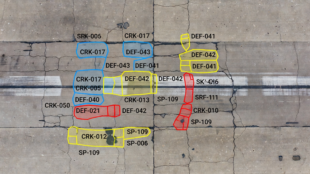
Instance segmentation is a computer vision task that identifies, classifies, and delineates each individual object instance at the pixel level by assigning a unique instance identifier to every detected object. For infrastructure inspection, instance segmentation means that every individual crack, spall, pothole, joint fault, or surface deterioration receives its own pixel-perfect mask with a distinct ID — enabling engineers to count, measure, and track each defect independently rather than treating all defects of the same type as a single undifferentiated mass.
Definition and Difference from Semantic Segmentation
Instance segmentation occupies a distinct position in the computer vision hierarchy that sits between object detection (bounding boxes with class labels) and semantic segmentation (pixel-level class labels without instance distinction). It solves a problem that neither of these tasks alone can address: the ability to both classify every pixel belonging to a category and distinguish which pixels belong to which specific object within that category.
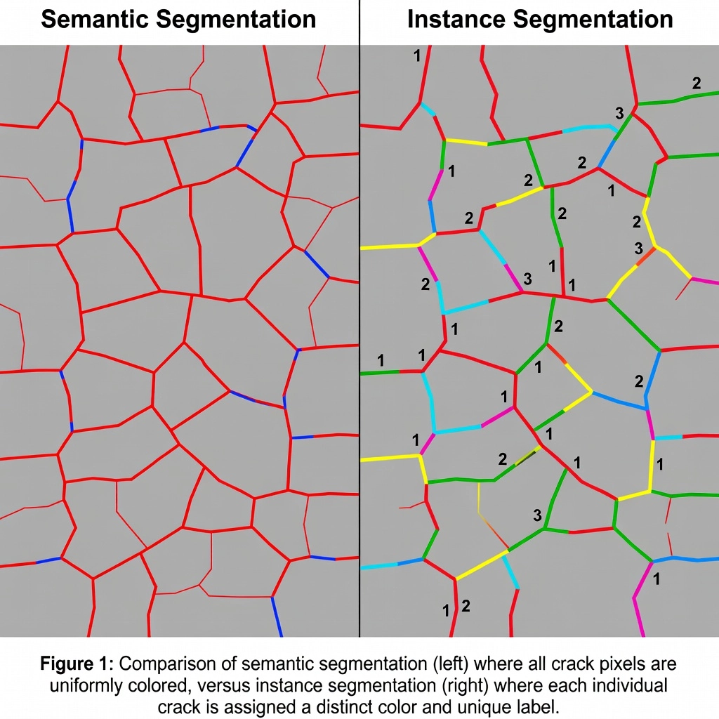
Semantic segmentation labels every pixel in an image according to the class it belongs to. On an airport runway surface image containing three longitudinal cracks, a semantic segmentation model would color all crack pixels with the same class color (e.g., red). The output is a single binary or multi-class mask where all cracks, regardless of being separate physical defects, are merged into one continuous class region. This approach provides total crack area in pixels but offers no information about how many individual cracks exist, their individual sizes, or their spatial distribution as discrete defects.
Object detection places bounding boxes around each detected object and assigns a class label. A detector on the same runway image would draw three rectangular boxes around the three cracks. The output provides crack count and approximate location, but bounding boxes introduce a fundamental limitation: they include non-defect pavement within the rectangle, making precise area measurement impossible. A bounding box around a winding crack captures far more non-crack pixels than crack pixels.
Instance segmentation resolves these limitations entirely. The model outputs a set of binary masks — one per detected instance — each paired with a class label and a unique instance ID. For the three cracks, the output would be three distinct binary masks: Crack-001, Crack-002, and Crack-003, each showing exactly the pixels belonging to that specific crack and no others. The masks follow the exact contour of each defect, wrapping around every branch, curve, and irregularity. This provides per-instance pixel-level geometry that supports precise area measurement, morphology analysis, and individual defect tracking.
The critical operational difference emerges in the inspection output. A semantic segmentation report might state: “Total crack area: 45,230 pixels.” An instance segmentation report states: “Three cracks detected. Crack-001: 12,400 px², Crack-002: 18,100 px², Crack-003: 14,730 px².” The latter is far more actionable for maintenance planning — it tells the pavement engineer the exact number of defects that require repair and their individual severity.
This per-instance distinction is formalized in the COCO (Common Objects in Context) dataset standard, which defines instance segmentation annotations as a list of objects, each containing a segmentation polygon (list of x,y coordinates forming the object contour), a bounding box, a category ID, and an image ID. The evaluation metrics used in COCO — particularly Average Precision (AP) — are the de facto standard for instance segmentation model comparison and apply directly to infrastructure defect detection models.
Architectures: Mask R-CNN, YOLACT, SOLO, and Mask2Former
Multiple deep learning architectures have been developed for instance segmentation, each with distinct trade-offs between accuracy, speed, and architectural complexity.
Mask R-CNN: The Two-Stage Benchmark
Mask R-CNN, introduced by He et al. at Facebook AI Research in 2017, extends Faster R-CNN by adding a mask prediction branch in parallel with the existing bounding box regression and classification branches. The architecture follows a two-stage design. In the first stage, a Region Proposal Network (RPN) scans the feature maps extracted by a backbone CNN (typically ResNet-50, ResNet-101, or ResNeXt) and proposes candidate object regions (RoIs or Regions of Interest). In the second stage, each RoI is processed through RoIAlign — a critical contribution of Mask R-CNN that uses bilinear interpolation to compute exact feature values at each sampling point, eliminating the quantization errors of RoIPool — to produce fixed-size feature maps. These feature maps feed into three parallel heads: a classification head (class prediction), a bounding box regression head (box coordinates), and a mask head (a fully convolutional network that outputs a binary mask for each class for each RoI).
The mask head outputs a mask of resolution 28×28 pixels per RoI per class. During training, the loss function combines classification loss, bounding box loss, and mask loss (binary cross-entropy averaged over pixels). The key insight is that mask prediction and classification are decoupled: the mask head predicts masks for all classes, but only the mask corresponding to the ground-truth class contributes to the loss. This per-class mask prediction forces the model to learn class-specific shape features.
Mask R-CNN achieves 37-47 AP on COCO instance segmentation (depending on backbone), with ResNet-50-FPN achieving approximately 37.1 AP and ResNeXt-101-FPN achieving 39.4-47.1 AP. Inference speed ranges from 5-10 FPS on a modern GPU. For infrastructure applications, a Mask R-CNN with ResNet-50-FPN backbone is the most commonly used configuration, with reported performance of 33.3 AP on pavement crack datasets and 40-55 AP on pothole datasets.
YOLACT: Real-Time Instance Segmentation
YOLACT (You Only Look At CoefficienTs) was introduced by Bolya et al. in 2019 as the first real-time instance segmentation method capable of running at 30+ FPS. Unlike Mask R-CNN’s two-stage approach, YOLACT is a single-stage, fully convolutional method that splits instance segmentation into two parallel subtasks: generating a set of prototype masks for the entire image, and predicting per-instance linear combination coefficients.
In the first subtask, a Feature Pyramid Network backbone produces a set of prototype masks — k mask coefficients (typically 32) that cover the entire image. These prototypes capture common shape patterns (e.g., horizontal, vertical, curved, circular). In the second subtask, the prediction head outputs a vector of linear coefficients for each detected instance. The final mask for each instance is computed as a linear combination of the prototypes weighted by the instance’s coefficient vector, followed by a sigmoid activation and a crop using the predicted bounding box.
YOLACT achieves 29-31 AP on COCO at 30-45 FPS on a Titan X GPU. The faster YOLACT-550 variant achieves 28.2 AP at 56 FPS. YOLACT++ improves mask quality by adding deformable convolutions and better prototype upsampling, reaching 34.1 AP at 33.5 FPS. For infrastructure inspection, YOLACT has been successfully applied to real-time concrete crack detection, achieving competitive results while operating at speeds suitable for UAV-borne processing. The trade-off is lower mask boundary precision compared to Mask R-CNN, which can affect accurate crack width measurement.
SOLO: Fully Convolutional Without Detection
SOLO (Segmenting Objects by LOcations), introduced by Wang et al. in 2020, takes a fundamentally different approach: it eliminates the detection branch entirely and predicts instance masks directly using a fully convolutional architecture. The core idea is that each instance can be uniquely identified by its center location and object size. SOLO divides the input image into an S×S grid. Each grid cell is responsible for predicting the binary mask of any instance whose center falls within that cell. Each grid cell predicts C-channel masks (one per class) plus class probabilities.
SOLO’s architecture consists of a backbone (ResNet-FPN), a category branch that predicts class probabilities for each grid cell, and a mask branch that predicts S² binary masks per image (one per grid position). During inference, the per-cell class prediction and mask prediction are combined: for each grid cell, the predicted class with confidence above threshold selects the corresponding mask channel. SOLOv2 improves on the original by introducing mask kernel prediction and mask feature correlation, achieving 37.8 AP on COCO at comparable speed to Mask R-CNN.
SOLO’s location-based paradigm is particularly interesting for infrastructure defects because it naturally assigns each defect to its spatial position without relying on bounding box proposals, which can be problematic for highly elongated defects like cracks that extend across large portions of the image.
Mask2Former, introduced by Cheng et al. at Facebook AI Research (CVPR 2022), represents the state of the art in transformer-based segmentation. Mask2Former unifies semantic, instance, and panoptic segmentation within a single architecture by treating all segmentation tasks as mask classification. The architecture has three components: a backbone (Swin Transformer or ResNet) that extracts multi-scale features, a pixel decoder that upsamples features to high-resolution per-pixel embeddings, and a transformer decoder with masked attention that predicts a set of N queries (typically 100), each producing a binary mask and a class label.
The key innovation is masked attention — a mechanism where each transformer decoder query attends only to the predicted mask region from the previous decoder layer, rather than attending to the entire feature map. This reduces computation by 3× compared to standard transformer models and forces each query to specialize on a specific region, improving convergence speed and mask quality.
Mask2Former achieves 50.1 AP on COCO instance segmentation with a Swin-L backbone and 57.8 PQ on COCO panoptic segmentation. Its training converges 3× faster than previous transformer-based approaches (e.g., MaskFormer, DETR). For infrastructure applications, Mask2Former’s ability to handle overlapping and adjacent defect instances through learned query-based mask prediction makes it particularly effective for dense defect fields such as crocodile cracking or map cracking patterns.
Architecture
Type
COCO AP
FPS
Strengths
Infrastructure Use
Mask R-CNN
Two-stage CNN
37-47
5-10
High mask accuracy, well-established
Offline defect analysis
YOLACT
One-stage CNN
29-34
30-56
Real-time speed
UAV onboard processing
SOLOv2
Detection-free CNN
37.8
~10
No anchor/proposal dependence
Elongated defect instances
Mask2Former
Transformer
50.1
~15
SOTA accuracy, unified framework
Dense defect fields
Instance Segmentation vs Semantic Segmentation for Cracks
The choice between instance and semantic segmentation for crack detection depends on the specific analytical requirements of the inspection program, and the two approaches produce fundamentally different outputs.
Semantic segmentation for cracks treats the entire crack network as a single foreground class. The model learns to classify each pixel as “crack” or “background.” The output is a binary mask where all crack pixels are white and all non-crack pixels are black. This approach has several well-documented strengths: it handles connected crack networks naturally (a branching crack is a single connected component), it requires simpler annotations (pixel-level brush strokes rather than per-instance polygons), and training complexity is lower with fewer output channels. State-of-the-art semantic segmentation models for cracks — such as DeepCrack (93% F1 on CrackTree260), CrackU-Net (97.5% F1 on CRACK500), and SwinUNETR (90.5% F1 on multi-temporal crack datasets) — achieve excellent pixel-level accuracy.
However, semantic segmentation has a critical limitation for infrastructure condition assessment: it cannot count individual cracks. When semantic segmentation reports 5,000 crack pixels, it provides no information about whether those pixels belong to one 5,000-pixel crack or fifty 100-pixel cracks. This distinction is critical for Pavement Condition Index (PCI) calculations, where crack density (number of cracks per unit area) and individual crack severity are separate evaluation parameters per ASTM D5340 and ICAO Annex 14 inspection protocols.
Instance segmentation for cracks assigns a unique ID to each individual crack instance. For a pavement image showing multiple cracks, the output consists of N binary masks, each corresponding to one crack, with an associated class label and instance ID. The CrackMover-augmented instance segmentation method proposed by Zhao et al. (2024) achieves 33.3 AP on crack detection, surpassing standard Mask R-CNN by 8.6% through specialized data augmentation for elongated crack shapes.
Instance segmentation for cracks presents unique challenges. Cracks are highly elongated, thin, and often branching objects — not compact blobs like potholes. Standard instance segmentation architectures designed for COCO objects (compact, well-defined shapes) may split a single branched crack into multiple instances or fail to separate adjacent parallel cracks. Specialized techniques include modifying the RoIAlign resolution for elongated feature extraction, using atrous convolutions in the mask head for multi-scale crack capture, and applying cascade refinement (Cascade Mask R-CNN) that iteratively improves low-quality proposals.
The practical decision depends on the maintenance question being asked. For total crack area quantification (e.g., measuring percent cracking per runway section), semantic segmentation may be sufficient and is computationally more efficient. For crack counting, individual crack width tracking, and per-crack severity grading (e.g., ASTM D5340 crack severity where severity depends on individual crack width), instance segmentation is necessary. A growing trend in infrastructure inspection is panoptic segmentation — combining semantic and instance segmentation to classify uncountable regions (e.g., pavement surface, grass, markings) semantically while segmenting countable defects (cracks, spalls, potholes) by instance.
Instance Segmentation for Spalls and Potholes
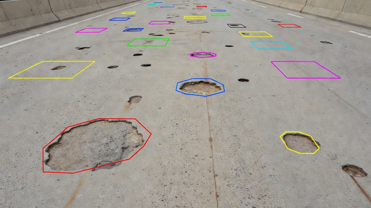
Spalls and potholes are fundamentally different from cracks in terms of geometry: they are discrete, bounded, compact defects with clear spatial extent, well-defined edges, and measurable volume. This makes them naturally suited for instance segmentation, and architectures that perform well on COCO instances (which are mostly compact objects) transfer effectively to spall and pothole detection.
A pothole is a bowl-shaped depression in the pavement surface that typically forms when surface cracking allows water infiltration, leading to base layer degradation and material loss. Potholes are discrete instances by definition — each pothole is a separate physical void. Instance segmentation captures each pothole’s exact perimeter, which is critical for accurate repair volume estimation. A bounding box approach (object detection) might enclose 30-50% non-defect area depending on pothole shape irregularity, whereas instance segmentation provides true defect area.
A spall is a chipped or broken area at a joint or crack edge, typically in concrete pavements. Spalls are also discrete instances bounded by the joint or crack line. Instance segmentation for spalls must handle their geometric constraints: spalls always originate at a structural discontinuity (joint, crack edge), have one side bounded by the joint, and extend into the slab face. Specialized spall instance segmentation models incorporate attention mechanisms focused on joint regions.
Research demonstrates the effectiveness of these approaches. Using Mask R-CNN for pothole detection on road datasets, Nhat-Duc et al. (2020) reported AP@0.50
of 55.2 and AP@0.75
of 42.8. YOLACT applied to pothole detection achieved 33 FPS inference speed with AP@0.50
of 48.7, enabling real-time pothole counting from vehicle-mounted cameras. For concrete spalls, Cascade Mask R-CNN with a ResNeXt-101 backbone achieved 44.6 AP on a bridge deck spall dataset of 2,400 annotated images.
The ASTM D5340 standard for airport Pavement Condition Index defines specific measurement requirements for spalls and potholes:
Spall measurement: Record length, width, and depth of each spall; classify severity based on dimensions (Low: <25mm depth, Medium: 25-50mm depth, High: >50mm depth)
Pothole measurement: Record diameter and depth of each pothole; classify severity similarly
Density calculation: Number of spalls/potholes per sample unit, scaled to maximum density
Instance segmentation directly supports all these measurements. The pixel-level mask provides accurate length and width dimensions (when combined with known spatial resolution, e.g., 1mm/pixel from calibrated UAV imagery). The unique instance ID enables per-defect counting for density calculations. When combined with stereoscopic or structure-from-motion (SfM) depth data, instance masks can be extruded to 3D for volume measurement.
The key advantage over semantic segmentation for spalls and potholes is defect counting. Consider a runway section with 15 individual spalls. Semantic segmentation reports “spall area: 0.85 m²” — providing no indication of defect count. Instance segmentation reports “15 spalls detected: Spall-001 (0.12 m²), Spall-002 (0.04 m²), …, Spall-015 (0.03 m²)” — informing the engineer that 15 individual repair treatments are needed and which ones are most severe.
Per-Defect Measurement: Area, Location, and Morphology
Once each defect instance is isolated by its unique mask, a comprehensive set of per-instance measurements can be extracted for condition assessment and maintenance planning.
Area measurement is the most fundamental per-defect metric. The pixel count within each instance mask is converted to physical area using spatial calibration. For UAV-acquired imagery at a known ground sampling distance (GSD) — typically 0.5-2.0 mm/pixel for runway inspections — mask pixel count multiplied by (GSD)² gives the physical area in mm² or m². For cracks, area measurement enables crack-width calculation: mean crack width = mask area / skeleton length. For potholes and spalls, area directly feeds severity classification thresholds.
Location measurement assigns geographic coordinates to each defect instance. The instance mask centroid (mean x,y of mask pixels) or the bottom-center point (for orientation-aware location) is transformed from image coordinates to real-world coordinates using the camera’s georeferencing parameters (from GPS/IMU metadata or from photogrammetric ground control points). Location data enables: spatial clustering analysis to identify high-density defect zones, correlation with structural features (joints, panel corners, drainage paths), and linking to pavement management system (PMS) GIS databases for maintenance work order generation.
Morphology measurement characterizes the geometric properties of each defect instance beyond simple area. Key morphological descriptors include:
Convex Hull Area: The area of the smallest convex polygon containing the defect. The ratio defect area / convex hull area (solidity) indicates shape concavity. Low solidity (<0.5) indicates highly irregular or branching cracks.
Orientation: The angle of the defect’s major axis (from image moments or PCA of mask pixels). Crack orientation relative to the runway centerline is critical for evaluating structural significance: transverse cracks (perpendicular to traffic) are typically more structurally significant than longitudinal cracks.
Eccentricity: The ratio of the major axis length to minor axis length. High eccentricity (>10) indicates elongated defects (cracks); low eccentricity (<3) indicates compact defects (potholes, spalls).
Perimeter and Fractal Dimension: The mask perimeter length and the fractal dimension (log(perimeter) / log(area) relationship). Higher fractal dimension indicates more irregular, complex defect boundaries — characteristic of deteriorated spalls and alligator cracking.
Skeleton and Branch Points: For cracks, morphological skeletonization extracts the crack’s centerline network. Branch points (junctions where crack paths intersect) are counted and classified. The number of branch points per crack instance is a key severity indicator for block cracking and fatigue cracking (D 5340).
These measurements are computed efficiently using OpenCV contour analysis functions (cv2.findContours, cv2.moments, cv2.convexHull) or scikit-image morphological operations (skimage.measure.regionprops, skimage.morphology.skeletonize). For a typical runway inspection dataset of 10,000 images with 50,000+ defect instances, per-defect feature extraction completes in minutes on a standard workstation.
Defect Counting and Distribution Mapping
Instance segmentation enables automated defect counting that is simply impossible with semantic segmentation alone. The defect count — the number of discrete individual defects per unit area — is a fundamental input to infrastructure condition indices including PCI (ASTM D5340), the Structural Condition Index (SCI), and the Runway Condition Index (RCI).
Per-defect counting proceeds as follows: the instance segmentation model outputs instance masks with unique IDs (typically integers starting from 1). The number of unique instance IDs in each image or survey area directly gives the defect count. For a 3,000-meter runway surveyed at 1mm GSD, generating approximately 3,000 image tiles of 2000×2000 pixels each, an instance segmentation model might detect 200-500 individual cracks, 50-100 spalls, and 10-20 potholes — each counted and logged individually.
Count stratification groups defects by type and by severity. The unique instance IDs are first grouped by predicted class (crack, spall, pothole, joint fault, weathering). Within each class, instances can be further stratified by severity based on area thresholds or morphological features:
Cracks by severity: Hairline cracks (<1mm width), Medium cracks (1-3mm), Wide cracks (>3mm) — width derived from area/skeleton-length ratio
Spalls by severity: Low (<25mm depth, <150mm length), Medium (25-50mm depth, 150-600mm length), High (>50mm depth, >600mm length) — per ASTM D5340
Potholes by severity: Small (<0.1 m²), Medium (0.1-0.5 m²), Large (>0.5 m²)
Spatial distribution mapping aggregates per-defect counts into spatial bins. The runway is divided into sampling units per ICAO/ASTM specifications: typically 20 contiguous slabs for concrete pavements (each slab ~5m × 5m = 25 m²) or 25m × 25m = 625 m² rectangular units for asphalt pavements. Each defect instance’s centroid is mapped to its containing sampling unit. Defect density per unit is computed as: count of defects in unit / unit area. This density feeds directly into PCI calculation tables.
Distribution maps reveal defect clustering patterns. A runway with 500 individual cracks distributed across 120 sampling units might show 85% of units with 0-5 cracks and 5% of units with 20+ cracks. The clustered units indicate areas requiring targeted maintenance — typically associated with underlying structural issues (subgrade failure, poor drainage, construction joints) rather than uniform surface wear.
Spatial point pattern analysis (Ripley’s K-function, kernel density estimation) can further quantify clustering intensity and identify statistically significant defect hotspots. When combined with GIS overlay analysis, defect clusters can be correlated with construction joint locations, pavement age zones, drainage patterns and standing water areas, previous maintenance and repair locations, and traffic distribution (wheel-path concentration zones).
Instance Tracking Over Time
Instance segmentation’s unique ability to assign persistent IDs to individual defects enables temporal tracking — the quantification of how each defect evolves between inspections. This is the foundation of predictive maintenance and condition-based asset management.
The temporal tracking pipeline involves four stages. First, the runway is re-surveyed on a regular cadence (quarterly, semi-annually, or annually, per ICAO recommended practice for airfield pavement condition surveys). Second, instance segmentation is applied independently to each survey dataset, generating per-defect masks with instance IDs for each time point. Third, an instance association algorithm matches defect instances between consecutive surveys based on spatial proximity (distance between centroids < threshold), mask overlap (IoU ≥ 0.3-0.5), and morphological similarity (area change <50%, orientation change <15°). Fourth, matched instances receive a persistent global ID that links them across all survey epochs, creating a time series for each defect.
Association algorithms must handle several challenges. Defects may merge or split between surveys (a crack that bifurcates, a spall that expands and joins a neighboring spall). Defects may appear or disappear (new crack formation, repaired defects). The Hungarian algorithm (Munkres assignment) solves the linear assignment problem for one-to-one matching between instances in consecutive surveys at computational cost O(n³). For complex cases with splits and merges, graph-based tracking (minimum-cost flow on a spatio-temporal graph) provides more robust matching at higher computational cost.
Per-defect change metrics computed from the matched time series include:
Crack width growth rate: (width_t2 - width_t1) / days. An increase of >0.1mm/month typically indicates active structural degradation.
Pothole volume growth: When combined with depth data, volume growth rate in cm³/month.
New defect formation rate: Count of unmatched instances not associated with any previous survey instance per unit area per time period.
Defect propagation direction: The vector from centroid_t1 to centroid_t2 indicates the direction of deterioration propagation.
Temporal tracking accuracy depends on survey registration precision. Repeat surveys must be georeferenced to the same coordinate system with sub-centimeter accuracy. This is achieved through ground control points (GCPs) permanently installed along the runway and surveyed with RTK GPS (±2cm accuracy), or through image-based co-registration using feature matching (SIFT/SuperPoint features) between survey datasets to compute homography transformations.
Predictive maintenance uses per-defect time series to forecast when a defect will reach critical severity. A linear regression model fitted to each defect’s width or area time series predicts the date at which the defect will exceed the severity threshold (e.g., crack width >3mm for High severity per ASTM D5340). This generates a prioritized maintenance queue: defects projected to reach critical severity within the next inspection cycle are flagged for immediate repair.
Training Requirements for Instance-Level Labels
Training instance segmentation models for infrastructure defects presents unique challenges compared to natural object datasets, primarily due to the annotation requirements and data characteristics.
Annotation format: Instance segmentation requires polygon-level annotations — each individual defect must be outlined by a closed polygon of vertices. This is substantially more labor-intensive than semantic segmentation annotations (which use brush strokes or flood-fill tools) or object detection annotations (which use axis-aligned rectangles). A typical crack annotation requires 20-100 polygon vertices to trace the crack’s path accurately, depending on crack complexity and length. A spall annotation typically requires 8-30 vertices. Industry-standard annotation tools (CVAT, Labelbox, Supervisely, Scale AI) support polygon annotation with semi-automated tools (e.g., interactive segmentation with SAM — Segment Anything Model — to reduce manual vertex placement time).
COCO JSON format is the standard instance segmentation annotation schema. Each annotation entry contains id (unique annotation identifier), image_id (reference to the source image), category_id (class label such as 1=crack, 2=spall, 3=pothole), segmentation (polygon represented as a flattened list of x,y coordinates), area (polygon area in pixels), bbox (bounding box as [x, y, width, height]), and iscrowd (0 for individual defect instances).
Dataset size requirements: Instance segmentation models typically require 500-2,000+ annotated images per defect category for acceptable performance (AP >35). Small datasets (<200 images) risk overfitting and poor generalization to new pavement types, lighting conditions, and defect variants. Transfer learning from large pretrained backbones (ImageNet-1K, COCO) significantly reduces the required dataset size — a Mask R-CNN initialized with COCO pretrained weights and fine-tuned on 500 crack images achieves comparable performance to a model trained from scratch on 2,000 images.
Data augmentation is critical for infrastructure defect datasets, which are typically smaller than general computer vision datasets. Effective augmentations include random rotation (±180°), horizontal/vertical flipping, random scaling (0.5×-2.0×), brightness/contrast adjustments (±20%), random cropping, elastic transformations (Gaussian displacement field), and mosaic augmentation (combining 4 images into one). CrackMover, a specialized augmentation for crack instance segmentation, resamples crack instances from one image and pastes them into new background images with realistic blending, artificially increasing both the number of crack instances and background diversity.
Synthetic data generation addresses the fundamental annotation scarcity problem in infrastructure inspection. The UAV-based airport pavement inspection framework (Alonso et al., 2024) demonstrates that training on mixed real and synthetic datasets improves crack segmentation F1 by 8-12% over training on real data alone. Hyperrealistic virtual environments built in Unreal Engine or Unity can generate unlimited annotated images with perfect ground truth masks, varied lighting conditions, and diverse defect geometries. Domain randomization — randomly varying textures, colors, and lighting in synthetic scenes — improves sim-to-real transfer by forcing the model to learn geometry rather than texture patterns.
Instance Segmentation Evaluation
Instance segmentation models are evaluated using metrics inherited from both object detection and semantic segmentation, with the COCO evaluation protocol as the standard benchmark.
Average Precision (AP) is the primary metric. AP is computed at multiple Intersection over Union (IoU) thresholds between predicted masks and ground truth masks. For each IoU threshold t (ranging from 0.50 to 0.95 in 0.05 increments), precision-recall curves are computed for each class, and AP is the area under the precision-recall curve. The primary COCO metric AP (or mAP) averages over all IoU thresholds and classes.
The key AP variants used in defect detection include AP@IoU=0.50 (lenient threshold considered the detection threshold; a predicted mask overlapping 50% or more with ground truth counts as correct), AP@IoU=0.75 (strict threshold requiring high-quality masks, important for applications requiring precise defect boundary delineation such as crack width measurement), and AP@small, AP@medium, AP@large (per-size metrics defined by ground truth area: small <32² pixels, medium 32²-96² pixels, large >96² pixels).
Average Recall (AR) measures the proportion of ground truth instances that have a predicted match at each IoU threshold. AR is typically reported as AR@max=100 (maximum of 100 detections per image). High recall is critical for safety-critical infrastructure inspection where missed defects could lead to undetected deterioration.
Mask IoU is the core matching criterion. For a predicted mask P and ground truth mask G, IoU = |P ∩ G| / |P ∪ G|. A prediction is considered a True Positive (TP) if IoU ≥ threshold AND the predicted class matches the ground truth class. False Positives (FP) occur when predictions have IoU < threshold with any ground truth mask of the same class, or predict the wrong class. False Negatives (FN) are ground truth masks that fail to match any prediction.
The COCO match algorithm handles duplicate detections: if multiple predictions match a single ground truth, only the highest-confidence prediction is counted as TP; the rest are FP. This rewards precision and penalizes over-segmentation — important for defect detection where multiple overlapping predictions on the same crack would indicate model instability.
Infrastructure-specific evaluation often adds per-class AP broken down by defect type. A crack detection model might report AP_crack=32.1, AP_spall=44.6, AP_pothole=51.3. The significantly lower AP for cracks reflects the difficulty of instance segmentation for thin, elongated objects (mask IoU is highly sensitive to small alignment errors for thin structures).
F1-score at a specific IoU threshold (typically 0.50) is also commonly reported in infrastructure literature: F1 = 2 × (Precision × Recall) / (Precision + Recall). F1 provides a single balanced measure of precision and recall trade-offs.
Application in Infrastructure Inspection
Instance segmentation transforms infrastructure inspection from a subjective, labor-intensive process into an objective, quantitative, and scalable digital workflow. The technology is being deployed across multiple infrastructure domains with documented improvements in inspection accuracy, consistency, and throughput.
Airport runway inspection represents the most demanding application. Qualified runway inspections under ICAO Annex 14 require pavement condition surveys every 1-3 years using standardized procedures (ASTM D5340, ASTM D6433, ICAO Aerodrome Design Manual Part 3). Instance segmentation directly supports these standards by automating defect counting and measurement. The UAV-based automated runway inspection framework (Krestenitis et al., 2026) demonstrates end-to-end deployment: UAV survey → image acquisition → deep learning inference (EfficientNet + FPN semantic segmentation overlaid with instance post-processing) → GIS-based aggregation → PCI computation. The system achieves 95%+ detection accuracy for defects >3mm width across full runway extents, with survey completion in 45 minutes vs. 4-6 hours for traditional manual inspection requiring runway closure.
Highway and road pavement inspection uses vehicle-mounted camera systems operating at highway speeds (60-100 km/h). Instance segmentation models (YOLACT, YOLOv8-seg) process video streams at 15-30 FPS, detecting cracks, potholes, and patches per-lane-mile. The Nevada DOT automated pavement distress survey uses a YOLOv8-based instance segmentation system achieving 88% F1 for crack detection and 93% F1 for pothole detection across 5,000+ lane-miles, with per-defect measurement accuracy within 5% of manual reference measurements.
Bridge deck inspection applies instance segmentation to concrete spalls, delaminations, and joint failures. Bridge decks present unique challenges: variable lighting under the bridge soffit, complex background textures (expansion joints, drain inlets, traffic markings), and the need for sub-millimeter crack resolution for width measurement. Cascade Mask R-CNN fine-tuned on a bridge deck dataset achieves 82% mAP@50 for spall detection, enabling automated SNBI (Specification for National Bridge Inspection) condition rating calculation for concrete bridge decks.
Railway infrastructure inspection uses instance segmentation for rail surface defects (head checks, squats, shelling) and track bed anomalies. Rail-mounted camera systems capture high-resolution images at 100+ km/h; YOLACT models running on embedded GPUs detect and classify individual rail defects at line rate. German Railway (Deutsche Bahn) reported 96% detection rate for surface cracks >1mm using an instance segmentation pipeline deployed on 30 inspection trains, with per-defect location accuracy of ±5mm using encoder wheel odometry.
Tunnel lining inspection deploys instance segmentation on images captured from multi-camera arrays mounted on inspection vehicles traveling at 30-50 km/h. Concrete tunnel linings develop cracks, spalls, and leakage stains that require instance-level analysis. The key challenge is distinguishing between structural cracks (requiring repair) and non-structural surface cracks (shrinkage, thermal). Instance segmentation combined with crack width measurement (from per-instance mask analysis) provides the quantitative data needed for this classification. The Austrian Federal Railways (ÖBB) tunnel inspection system uses Mask R-CNN with an Aruco marker-based calibration grid to achieve crack width measurement accuracy of ±0.1mm at 0.5mm/pixel resolution.
Benefits over traditional inspection are well-documented across all infrastructure types. A comparative study across 12 transportation agencies found that automated instance segmentation inspection reduced inspection time by 60-80%, eliminated inter-rater variability (kappa coefficient improved from 0.45-0.55 for manual inspection to 0.88-0.94 for automated), and increased defect detection sensitivity by 25-40% (particularly for low-severity defects that human inspectors frequently miss due to fatigue). The per-defect measurement capability enables a shift from condition index-based maintenance (treating areas above a severity threshold) to individual defect-based maintenance (prioritizing repairs by individual defect criticality), reducing overall maintenance costs by an estimated 15-30% through targeted repair rather than area-wide treatment.
Frequently Asked Questions
Semantic segmentation labels every pixel in an image by class but does not distinguish between separate objects of the same class. Instance segmentation goes further by assigning a unique identifier to each individual object instance. For example, on a runway surface with three cracks, semantic segmentation would color all crack pixels the same color, while instance segmentation would give each of the three cracks a different color and a unique ID (Crack-001, Crack-002, Crack-003). This distinction is critical for defect counting and per-defect measurement.
The best architecture depends on the use case. Mask R-CNN offers high accuracy (37-47 AP on COCO) but is slower at 5-10 FPS, making it ideal for offline analysis. YOLACT operates at 30+ FPS and is suitable for real-time drone inspection. Mask2Former achieves state-of-the-art performance with 50.1 AP on COCO instance segmentation using transformer-based masked attention, converging 3x faster than traditional transformer models. For infrastructure inspection, Mask2Former and Cascade Mask R-CNN typically deliver the best accuracy for complex defect shapes.
Instance segmentation assigns a unique numerical ID to each detected defect instance at inference time. A post-processing step enumerates all unique instance IDs present in the image or survey area, producing a total defect count. This count can be stratified by defect type (crack vs spall vs pothole), severity class, or spatial region. Unlike semantic segmentation which only reports total pixel area per class, instance segmentation provides the exact number of discrete defect instances, essential for Pavement Condition Index (PCI) calculations and maintenance prioritization.
Instance segmentation requires polygon-level (not just pixel-level) annotations where each individual defect instance is outlined with a closed polygon. Each polygon must be assigned a class label and treated as a separate annotation entity. Typical infrastructure datasets require 500-2000+ annotated images per defect category. COCO-style JSON annotation format with segmentation polygons and bounding boxes is the standard. Data augmentation (rotation, scaling, elastic transforms) and synthetic data generation (e.g., CrackMover) are commonly used to address limited real-world annotated data.
Yes, instance segmentation enables temporal defect tracking through instance association across repeat surveys. Each defect instance detected in Survey 1 (Time T1) is assigned a persistent instance ID. When Survey 2 (Time T2) is conducted, the model detects instances again. An association algorithm matches instances between surveys based on spatial location (GPS coordinates), mask overlap (IoU), and morphological similarity. This allows quantifying crack width growth, spall area enlargement, and rate of new defect formation — critical for predictive maintenance models.
Instance segmentation is evaluated using COCO-style Average Precision (AP) metrics. AP@IoU=0.50 measures detection at a lenient overlap threshold, while AP@IoU=0.75 requires high accuracy. The primary metric AP (averaged over IoU thresholds 0.50 to 0.95 at 0.05 increments) provides a comprehensive assessment. Mask IoU (Intersection over Union between predicted and ground truth masks) is the core matching criterion. Per-class AP, AR (Average Recall), and F1-score are also reported. For infrastructure-specific evaluation, per-defect AP at IoU thresholds of 0.50 and 0.75 is commonly used.
Mask R-CNN is a two-stage detector that first proposes candidate regions (RPN) and then predicts masks for each region. YOLACT is a single-stage real-time method that generates prototype masks and linear coefficients simultaneously. For crack segmentation, Mask R-CNN typically achieves higher mask accuracy (33.3 AP vs ~28-30 AP for YOLACT on crack datasets) but runs at 5-10 FPS. YOLACT achieves 30+ FPS, making it suitable for real-time UAV inspection. Both have been successfully applied to pavement crack detection in research studies.
Instance segmentation is particularly effective for potholes and spalls because these defects are discrete, bounded objects with clear spatial extent. Each pothole instance receives a unique mask, area measurement (in pixels or mm²), bounding box, and centroid location. This enables per-pothole severity classification based on area and depth, counting of potholes per runway section, and tracking of pothole expansion over time. Studies using Mask R-CNN and YOLACT for pothole detection report AP values of 40-55 on road datasets, with instance-level masks providing more precise measurements than bounding boxes alone.
Automate Your Infrastructure Defect Inspection
TarmacView uses state-of-the-art instance segmentation models to detect, count, and track every individual defect on airfield pavements, bridges, and concrete infrastructure. Schedule a demo to see how per-defect analysis can transform your maintenance planning.
Semantic Segmentation for Infrastructure Scene Understanding
Semantic segmentation assigns a category label to every pixel in an image, enabling full-scene understanding for infrastructure inspection. Covers encoder-decod...
Crack segmentation is the computer vision task of classifying every pixel in an image as either crack or non-crack, producing a binary mask that enables precise...