Inertial Profiler
A vehicle-mounted inertial profiler uses laser height sensors and accelerometers to measure longitudinal pavement profile at highway speeds, computing IRI and r...
27 min read
Pavement Testing
Pavement Smoothness
+2
The International Roughness Index (IRI) is a standardized longitudinal profile-based measure of pavement roughness, expressed in m/km or in/mi. Developed by the World Bank, IRI is the most widely used pavement smoothness metric globally. Covers calculation from profile data, relationship to ride quality and vehicle operating costs, measurement equipment, and estimation from drone imagery.
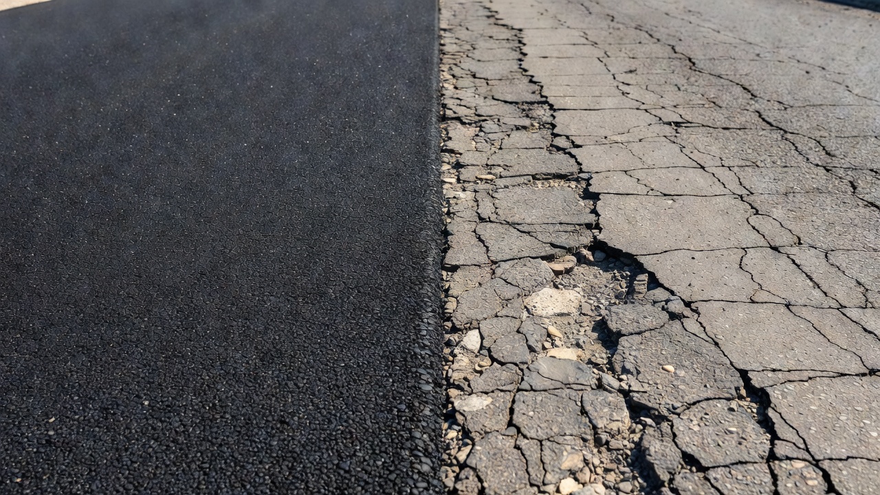
The International Roughness Index (IRI) is a standardized, mathematically rigorous measure of the longitudinal road profile that quantifies pavement surface roughness. It is defined as the accumulated suspension stroke of a reference quarter-car vehicle traveling at 80 km/h, divided by the distance traveled, yielding a dimensionless slope value typically expressed in meters per kilometer (m/km), millimeters per meter (mm/m), or inches per mile (in/mi). The conversion is 1 m/km = 63.36 in/mi. In its essence, an IRI of 0.0 represents a perfectly smooth surface, while higher values indicate progressively rougher roads. Unlike subjective ride quality ratings, IRI is purely a mathematical function of the measured elevation profile and the standardized vehicle simulation parameters defined in ASTM E1926 and AASHTO PP 37, making it repeatable, reproducible, and time-stable across different measurement devices, operators, and time periods.
The technical definition found in ASTM E867 defines roughness as “the deviation of a surface from a true planar surface with characteristic dimensions that affect vehicle dynamics and ride quality.” IRI operationalizes this definition by filtering longitudinal profile wavelengths that are relevant to vehicle response — specifically wavelengths between approximately 0.5 meters and 91 meters (0.5 feet to 300 feet). Shorter wavelengths correspond to pavement texture and megatexture, which affect tire-pavement noise and friction but not ride quality. Longer wavelengths correspond to grade changes and topography, which are not considered roughness. The IRI isolates the range of wavelengths that produce perceptible vertical acceleration in passenger vehicles, making it directly relevant to both the physical vehicle response and the subjective human perception of ride quality.
The IRI is an open-ended scale with no theoretical upper bound, though practical values on paved roads rarely exceed 12 m/km (760 in/mi), which would correspond to an extremely deteriorated, nearly impassable surface. The IRI value is expressed as a summary statistic — typically the mean IRI computed over a defined segment length, commonly 100 meters or 0.1 mile (160 meters) for highway applications. For airport runway applications, the reporting interval is often shorter, at 30 meters or 100 feet, to capture local roughness events such as isolated bumps, dips, or faulted slabs that can induce critical aircraft dynamic responses at high takeoff and landing speeds.
The IRI emerged from a landmark international research program initiated by the World Bank in the late 1970s and early 1980s. The World Bank, as a major financier of road infrastructure projects in developing countries, needed an objective, equipment-independent method to evaluate road roughness for project prioritization, economic analysis, and performance monitoring. Prior to IRI, roughness measurement was fragmented across dozens of incompatible indices — each tied to specific measurement equipment or subjective rating procedures that could not be compared across borders.
The foundational research was conducted through the International Road Roughness Experiment (IRRE) held in Brasília, Brazil, in 1982. This experiment brought together road roughness measurement equipment from multiple countries — including response-type road roughness meters (RTRRMs), profilographs, and rod-and-level survey teams — to collect data on the same set of test sections covering a wide spectrum of roughness conditions, from newly constructed pavements to severely deteriorated gravel roads. The data from IRRE allowed researchers led by Michael W. Sayers, Thomas D. Gillespie, and Cesar A.V. Queiroz at the University of Michigan Transportation Research Institute (UMTRI) to develop a reference index that could serve as a common denominator for all existing roughness measurement methods.
The analytical foundation for IRI drew significantly from earlier work performed for the National Cooperative Highway Research Program (NCHRP) in the United States. NCHRP Project 1-10 and subsequent studies had developed the concept of using a quarter-car simulation model to characterize pavement profile, building on the quarter-car response theory that had been extensively studied in vehicle dynamics research. The NCHRP work identified that a standardized quarter-car model with fixed parameters — the so-called “Golden Car” — could produce a consistent roughness index from any elevation profile, regardless of how that profile was measured.
The IRI was formally established in 1986 with the publication of World Bank Technical Paper Number 46, “Guidelines for Conducting and Calibrating Road Roughness Measurements,” authored by Sayers, Gillespie, and Paterson. This seminal document provided the complete mathematical specification of the quarter-car simulation, the IRI calculation algorithm, calibration procedures for response-type meters, and guidelines for field data collection. The publication coincided with and supported the World Bank’s Highway Design and Maintenance Standards Model (HDM-III), which used IRI as a primary input to predict vehicle operating costs, road deterioration rates, and the economic benefits of pavement maintenance investments.
The adoption trajectory of IRI was accelerated by several factors. The FHWA Highway Performance Monitoring System (HPMS) adopted IRI as its standard roughness metric in the early 1990s, requiring all U.S. states to report pavement roughness in IRI units. The Long-Term Pavement Performance (LTPP) program, launched in 1987 as part of the Strategic Highway Research Program (SHRP), standardized on IRI for all its profile measurements across more than 2,000 test sections in North America. The AASHTO subsequently published standard specifications for IRI measurement (PP 37) and profile measurement (R 56), while ASTM International published E1926, “Standard Practice for Computing International Roughness Index of Roads from Longitudinal Profile Measurements,” which provides the definitive open-source algorithm specification.
The IRI is computed using a quarter-car mathematical model, which simulates the dynamic response of one corner — one quarter — of a passenger vehicle traveling over a measured road profile. The quarter-car model represents a simplified mechanical system consisting of two masses connected by springs and dampers: a sprung mass representing the portion of the vehicle body supported by the suspension at one corner, and an unsprung mass representing the wheel, tire, and axle assembly. The sprung mass is connected to the unsprung mass through a suspension spring and damper, while the unsprung mass contacts the road surface through a tire modeled as a linear spring.

The standardized “Golden Car” parameters used in the IRI simulation are:
| Parameter | Symbol | Value |
|---|---|---|
| Sprung mass per corner | m_s | 250 kg |
| Unsprung mass per corner | m_u | 37.5 kg |
| Suspension spring rate | k_s | 15.8 kN/m |
| Suspension damping coefficient | c_s | 1.0 kN·s/m |
| Tire spring rate | k_t | 158 kN/m |
| Tire damping coefficient | c_t | 0.0 kN·s/m |
| Mass ratio (m_u / m_s) | μ | 0.15 |
| Simulation speed | v | 80 km/h (22.22 m/s) |
The motion of the quarter-car system is governed by two coupled second-order differential equations. The first equation describes the vertical motion of the sprung mass, driven by the suspension spring and damper forces. The second equation describes the motion of the unsprung mass, driven by both the suspension forces and the tire spring force reacting to the road profile input. The road profile elevation at each longitudinal position serves as the base excitation input to the tire spring, and the equations are solved numerically at discrete time steps corresponding to the spatial sampling interval of the measured profile divided by the simulation speed.
The critical output of the simulation is the relative velocity between the sprung and unsprung masses, representing the rate at which the suspension is compressing or extending. The absolute value of this relative velocity is accumulated over the entire profile length and divided by the total distance traveled to yield the Average Rectified Slope (ARS). Mathematically:
ARS = (1/L) × ∫|v_s(t) − v_u(t)| dt
where L is the total profile length, v_s is the sprung mass vertical velocity, v_u is the unsprung mass vertical velocity, and the integration is performed over the travel time. The IRI is then obtained by multiplying the ARS by 1,000 to express it in convenient units:
IRI (m/km) = ARS × 1,000
The ARS is fundamentally a measure of suspension working travel per unit distance. A perfectly smooth road produces zero relative velocity between the masses, yielding IRI = 0. In practice, even the smoothest pavements have some residual texture and construction-induced variations that produce small but non-zero IRI values, typically in the range of 0.5 to 1.5 m/km (30 to 95 in/mi) for newly constructed high-quality asphalt or concrete surfaces.
The choice of 80 km/h as the simulation speed is significant. This speed represents the typical operating speed on major highways and produces suspension responses that correlate well with subjective ride quality ratings. At lower speeds, smaller-wavelength roughness features produce less dynamic excitation, while at higher speeds, the same features produce greater suspension travel and higher IRI. The IRI algorithm applies a moving average filter to smooth the profile before simulation, with a baseline length of 250 mm for profile sampling intervals of 25 mm or less. For larger sampling intervals, the baseline filter length is adjusted proportionally. This filtering removes the effect of microtexture and macrotexture, which are not relevant to ride quality.
It is important to understand that IRI is computed independently for each wheelpath. For equipment that measures both left and right wheelpaths simultaneously, the IRI is calculated separately for each profile and then averaged to obtain the mean IRI for the lane. Some agencies also report the maximum of the two wheelpath IRIs to capture the worst-case condition. The quarter-car model is inherently linear, meaning IRI scales proportionally with profile amplitude — doubling the amplitude of all deviations in the profile approximately doubles the IRI — a property that makes IRI well-suited for comparing roughness across different pavement types and construction methods.
The standardized procedure for computing IRI from a longitudinal profile is specified in ASTM E1926, “Standard Practice for Computing International Roughness Index of Roads from Longitudinal Profile Measurements.” The standard is reaffirmed periodically with the most recent reaffirmation in 2021. ASTM E1926 provides the complete algorithmic specification and reference implementation for processing any measured longitudinal elevation profile into an IRI value, ensuring that calculations performed by different software packages on the same profile data produce identical results.
The calculation proceeds through several stages. First, the raw elevation profile must be pre-processed to ensure it meets input requirements. The profile must have a constant sampling interval, typically between 25 mm and 300 mm (1 to 12 inches), with 25 mm being the most common for inertial profiler data. Any missing data points or gaps in the profile must be addressed through interpolation or segment exclusion. The profile length must be a minimum of 11 meters in addition to the segment of interest to accommodate the quarter-car model start-up transient — the first 11 meters of simulation output are discarded because the model requires distance to reach a steady-state response independent of arbitrary initial conditions.
The algorithm then applies a moving average filter to the profile. The filter baseline length is 250 mm for sampling intervals up to 25 mm, meaning that for 25 mm sampling, a 10-point moving average is used. For larger sampling intervals, the baseline length is set equal to the sampling interval, effectively meaning no smoothing is applied for intervals exceeding 250 mm. This filter removes high-frequency profile components corresponding to texture rather than roughness.
The filtered profile is then used to drive the quarter-car simulation. The governing differential equations are solved numerically using a recurrence formula that is computationally efficient and stable. The standard specifies a fourth-order Runge-Kutta integration scheme as the reference method, though simpler approaches such as the Euler method can be used if the sampling interval is sufficiently small. The recurrence formula processes the profile point by point, updating the state variables (sprung mass displacement and velocity, unsprung mass displacement and velocity) at each step based on the current profile elevation.
For each integration step, the absolute value of the relative velocity between sprung and unsprung masses is computed and accumulated. After processing the entire profile, the accumulated sum is divided by the total simulated travel distance (profile length minus the 11-meter start-up segment) and multiplied by 1,000 to produce the IRI in m/km. The standard also specifies how to handle segmented profiles — a long profile can be divided into overlapping segments with the IRI computed independently for each segment to produce a continuous roughness profile along the road.
A critical validation requirement in ASTM E1926 is that any software implementation must be verified against the reference profiles and known IRI values provided in the standard’s appendix. These validation profiles cover a range of roughness levels and profile characteristics, and the computed IRI must match the reference value within a specified tolerance of 0.1%. This ensures consistency across different software packages, equipment manufacturers, and agency implementations. Several validated open-source implementations exist, including ProVAL (Profile Viewing and Analysis software) developed by FHWA, which is freely available and widely used by state highway agencies for IRI computation and profile analysis.
The required profile accuracy for meaningful IRI computation depends on the application. For network-level condition surveys, a vertical accuracy of ±0.5 mm and a longitudinal accuracy of ±0.05% of the traveled distance are typical. For construction acceptance testing, more stringent accuracy requirements of ±0.25 mm vertically are common. The spatial frequency content of the profile — the wavelengths present — is what determines IRI, so the measurement system must accurately capture wavelengths from approximately 0.5 m to 91 m. Systems that attenuate or amplify specific wavelength ranges will produce biased IRI values, which is why equipment certification against reference profiles is essential.
The IRI can be measured using several classes of equipment, each with distinct capabilities, accuracy characteristics, and operational constraints. The choice of equipment depends on the application — whether it is network-level condition assessment, project-level construction acceptance, calibration verification, or research.
Inertial profilers are the predominant equipment class for highway-speed IRI data collection. These systems are mounted on survey vehicles — typically vans or SUVs — and operate at traffic speeds of 50 to 110 km/h (30 to 70 mph). An inertial profiler integrates three core sensor subsystems: a laser height sensor (or array of sensors) that measures the distance from the vehicle to the pavement surface at high frequency, an accelerometer that measures the vertical acceleration of the vehicle body to compensate for vehicle body motion, and a distance measurement instrument (DMI) that provides precise longitudinal position referencing. The raw sensor data is processed through a signal integration algorithm that subtracts the double-integrated accelerometer signal from the laser height measurement to recover the true pavement elevation profile independent of vehicle bounce, pitch, and roll.
Modern inertial profilers are specified under ASTM E950 / AASHTO R 56, “Standard Practice for Measuring the Longitudinal Profile of Traveled Surfaces with an Accelerometer-Established Inertial Profiling Reference.” These standards specify sensor performance requirements (accelerometer resolution ≤ 1 µg, laser resolution ≤ 0.025 mm, sampling interval ≤ 25 mm), operational protocols (minimum warm-up time, speed constraints, temperature ranges), and validation procedures. The profiler must demonstrate its accuracy on reference profiles with known IRI values, typically at certification tracks established by state highway agencies. The FHWA and AASHTO jointly developed a profiler certification process where profilers are tested on multiple pavement sections with varying roughness levels, and the measured IRI must fall within ±5% of the reference value on each section.
Inertial profilers capture profiles in each wheelpath simultaneously using dual laser sensors. The computed IRI for each wheelpath is averaged to report the lane IRI. High-end profilers may include additional sensors such as a longitudinal profile sensor for cross-slope measurement, texture lasers for macrotexture (Mean Profile Depth), and right-of-way cameras for imaging distresses. The cross-correlation between left and right wheelpath IRI values on typical highways is approximately 0.85 to 0.95, reflecting the fact that both wheelpaths experience similar construction and traffic loading but may have different localized distress patterns — particularly rutting in the right wheelpath from heavy truck channelization.
Walking profilers are manually operated, low-speed precision instruments that provide the highest accuracy reference measurements for IRI. The most recognized device in this class is the Dipstick (Face Companies), which consists of an inclinometer enclosed in a case supported by two legs spaced exactly 305 mm (12 inches) apart. The operator walks the device along a pre-marked line, pivoting it alternately about each leg, with the built-in inclinometer measuring the elevation difference between successive foot positions. The device records 10 to 15 readings per minute and can survey approximately 150 meters per hour with a single operator. The accumulated elevation differences are processed into a continuous profile with a vertical accuracy of ±0.127 mm (±0.005 inches).
Walking profiler data serves as the gold standard for certifying inertial profilers. State DOTs and research organizations establish calibration and certification tracks where the reference IRI is determined by walking profiler — or in some cases, by rod-and-level survey — and inertial profilers are then evaluated against these reference values. The walking profiler is also used for project-level acceptance testing on short pavement segments where the precision of high-speed profilers may be insufficient, and for research studies requiring the highest possible accuracy in profile measurement.
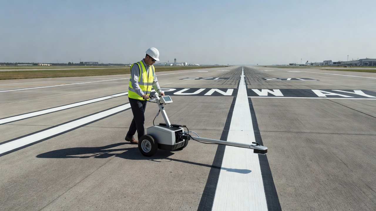
Road profilers represent a broader category that includes both high-speed inertial profilers and lower-speed devices designed for project-level surveys. A notable subcategory is the lightweight profiler, which can be mounted on a small trailer or carried by hand and pushed at walking speed. These devices use similar laser-accelerometer technology as full inertial profilers but in a lighter, more portable form factor. They are particularly useful for measuring short pavement sections, airport runways where vehicle access may be restricted, and urban streets with frequent stops. The SurPRO and Walking Profiler SSI are examples of commercially available lightweight devices that produce IRI data meeting ASTM E950 accuracy requirements.
Response-type meters measure the vertical movement of a vehicle body relative to its axle as the vehicle travels over the road. These devices — historically the most common roughness measurement method before inertial profilers became affordable — produce an output in counts per mile or a similar unit that correlates with roughness but is vehicle-specific and speed-dependent. Their primary limitation is that they do not directly measure the elevation profile; instead they measure the vehicle’s filtered response to that profile, which depends on the vehicle’s suspension characteristics, loading, tire pressure, and speed. RTRRMs must be calibrated to IRI using correlation equations developed by operating the response-type vehicle over calibration sections with known IRI values. While response-type devices are still used in some countries for network surveys due to their lower capital cost, the global trend is toward inertial profilers that provide direct profile measurements.
For HPMS reporting, FHWA requires that roughness data be collected using equipment that measures longitudinal profile in accordance with ASTM E950 and computes IRI per ASTM E1926. Response-type measurements alone are not sufficient unless they are correlated to profile-derived IRI through a documented calibration procedure, and even then the correlation must be updated periodically and cannot replace profile measurement on higher-level road systems.
Highway agencies classify pavement condition into categories based on IRI thresholds that reflect both ride quality and the need for maintenance intervention. The most widely referenced thresholds are those established by the Federal Highway Administration (FHWA) for the U.S. National Highway System (NHS), which define two primary condition levels:
| Condition Category | IRI (in/mi) | IRI (m/km) | Description |
|---|---|---|---|
| Good | ≤ 95 | ≤ 1.50 | Smooth ride; no corrective action required |
| Acceptable | 96–170 | 1.51–2.68 | Perceptible roughness but still within acceptable limits |
| Poor | > 170 | > 2.68 | Significant roughness; rehabilitation may be warranted |
FHWA established the 95 in/mi threshold as its primary performance target for the NHS, with the goal of increasing the percentage of vehicle-miles-traveled on pavements with IRI ≤ 95 in/mi. The 170 in/mi threshold serves as the minimum acceptable condition; pavements exceeding this value are considered to have deficient ride quality requiring attention. These FHWA thresholds are incorporated into the Highway Performance Monitoring System (HPMS) reporting requirements and are used in the FHWA Conditions and Performance Report to Congress.
Many state DOTs have adopted finer classification schemes. A typical five-category system used by several states is:
| Category | IRI (in/mi) | IRI (m/km) | Typical Ride Quality |
|---|---|---|---|
| Excellent | < 60 | < 0.95 | Like-new condition |
| Good | 60–94 | 0.95–1.49 | Minor imperfections |
| Fair | 95–170 | 1.50–2.68 | Noticeable roughness |
| Mediocre | 170–220 | 2.69–3.47 | Uncomfortable at highway speed |
| Poor | > 220 | > 3.47 | Rehabilitation needed |
For newly constructed pavements, the typical IRI values achieved depend on pavement type, construction quality control, and specification requirements. New hot-mix asphalt (HMA) pavements constructed under modern smoothness specifications typically achieve mean IRI values between 30 and 65 in/mi (0.5–1.0 m/km), with premium construction achieving values below 30 in/mi. New jointed plain concrete pavements (JPCP) typically achieve 40 to 80 in/mi (0.6–1.3 m/km) due to the inherent roughness introduced at transverse joints. Continuously reinforced concrete pavements (CRCP) can achieve values comparable to asphalt because they lack transverse joints.
The roughness progression rate — how quickly IRI increases over time — depends on traffic loading, environment, pavement structure, and maintenance history. Typical annual IRI increases range from 0.02 to 0.15 m/km (1 to 10 in/mi) for well-designed and well-constructed pavements under moderate traffic. Pavements with structural deficiencies, poor drainage, or extreme freeze-thaw exposure can deteriorate much more rapidly, with annual IRI increases exceeding 0.3 m/km (19 in/mi). This deterioration rate is a primary input to pavement management system predictions of future condition and treatment timing.
For gravel and unpaved roads, IRI thresholds are substantially higher because the expected roughness is greater even for well-maintained surfaces. The World Bank guidelines for unpaved roads classify IRI values below 6 m/km (380 in/mi) as good for earth roads, 6–10 m/km as fair, and above 10 m/km as poor. These higher thresholds reflect the different expectations for low-volume unpaved roads compared to paved highways, as well as the much higher vehicle operating costs associated with rough gravel surfaces.
IRI does not exist in isolation as a pavement performance measure — it complements and interacts with other established indices, particularly the Present Serviceability Index (PSI) and the Pavement Condition Index (PCI). Understanding these relationships is essential for agencies transitioning between condition rating systems or integrating IRI into existing pavement management frameworks.
The Present Serviceability Index (PSI) was developed during the AASHO Road Test conducted near Ottawa, Illinois, between 1958 and 1960 — the largest controlled pavement experiment ever undertaken. The road test established the concept of “serviceability” as the ability of a pavement to serve traffic, measured subjectively by a panel of raters who drove over test sections and assigned ratings on a scale of 0 to 5 (the Present Serviceability Rating, PSR). PSR was then correlated with objective physical measurements of the pavement — including roughness (measured by slope variance from CHLOE profilometer), cracking, patching, and rut depth — to produce the PSI equation:
PSI = 5.03 − 1.91 × log(1+SV) − 1.38 × RD² − 0.01 × √(C+P)
where SV is the slope variance (a measure of longitudinal roughness), RD is the mean rut depth in inches, C is the cracked area in square feet per 1,000 square feet, and P is the patched area. This equation shows that roughness (SV term) is the dominant contributor to PSI, but distresses such as cracking and patching also influence the rating.
When IRI was introduced in the 1980s, correlations were established to convert between IRI and PSI. Paterson (1986) proposed the exponential relationship:
PSI = 5 × e^(−IRI/5.5)
where IRI is in m/km. Al-Omari and Darter (1992), using data from five U.S. states on both flexible and rigid pavements, proposed an alternative correlation:
PSI = 5 × e^(−0.26 × IRI)
with IRI in m/km, achieving R² = 0.73 and a standard error of estimate of 0.39 PSI units. The differences between these two correlations reflect the sensitivity of PSI-IRI relationships to the specific pavement types, distress conditions, and rating panel characteristics.
An important conceptual distinction is that PSI is a multi-factor index incorporating cracking, rutting, and patching, while IRI is exclusively a roughness index. A pavement section can have a high PSI (good rating) but a relatively high IRI if the road is rough but has no visible cracking or rutting — as can occur with certain types of subgrade-related roughness. Conversely, a pavement with severe cracking but remained smooth due to recent crack sealing could have a low IRI but a low PSI. The correlation is therefore approximate and pavement-type-dependent. Modern pavement management increasingly treats IRI and PCI as complementary rather than competing indicators — IRI captures the functional condition (ride quality), while PCI captures the structural and surface condition (distress-based deterioration).
The Pavement Condition Index (PCI) is a numerical rating from 0 (failed) to 100 (excellent) based on the type, severity, and density of surface distresses present on the pavement. Developed by the U.S. Army Corps of Engineers and standardized in ASTM D6433, PCI is a visual survey index calculated by deducting points for each observed distress based on its extent and severity. Unlike IRI, which requires specialized measurement equipment, PCI can be determined through a visual walk-through or windshield survey.
The relationship between PCI and IRI is inherently nonlinear and pavement-type dependent. Research has shown that: for flexible pavements, IRI tends to remain relatively stable until PCI drops below approximately 50-60, after which IRI increases rapidly as structural distresses (fatigue cracking, rutting) begin to affect ride quality; for rigid pavements, IRI may increase earlier as joint faulting and spalling create localized roughness events that affect ride quality before PCI indicates widespread deterioration.
A generalized relationship has been observed where PCI = 100 − a × IRI^b, with parameters a and b calibrated to local conditions and pavement types. Some agencies use IRI as a screening trigger for more detailed PCI surveys — if IRI exceeds a threshold (e.g., 150 in/mi), a full PCI survey is triggered to determine the specific distress mechanisms and appropriate treatment — rather than relying on IRI alone for treatment selection.
Runway and taxiway roughness assessment represents a specialized application domain where IRI is used alongside other metrics tailored to aircraft dynamic response. The critical difference between highway and airport IRI applications is the aircraft speed and dynamic characteristics. While highway IRI is based on a passenger car traveling at 80 km/h, aircraft operate on runways at speeds from 0 to over 300 km/h (for takeoff and landing), with substantially different suspension characteristics, tire properties, and fuselage dynamics.
ICAO Annex 14, Volume I stipulates that the surface of newly constructed runways should not exhibit irregularities that impair aircraft operations. The traditional compliance method specified in Annex 14 is the 3-meter straightedge test — when a 3-meter straightedge is placed on the runway surface, the maximum deviation at any point should not exceed 3 mm for new construction. This is a localized roughness criterion that captures isolated bumps, dips, and grade changes but does not provide an overall smoothness index comparable to IRI. The 3-meter straightedge tolerance, while widely enforced, has recognized limitations: it cannot characterize longer-wavelength roughness features (such as gentle undulations over tens of meters) that can excite aircraft heave and pitch modes at high speeds.
The FAA Airport Pavement Roughness Research Program at the National Airport Pavement Test Facility (NAPTF) and the FAA Airport Technology R&D Branch has investigated the application of IRI to runways and developed supplemental roughness evaluation methods. FAA Advisory Circular AC 150/5380-9, “Guidelines and Procedures for Measuring and Evaluating Runway Roughness,” recommends using a continuous profile-measuring device (inertial profiler) to collect elevation data along runway wheelpaths and evaluate roughness using both IRI and Boeing Bump Index (BBI).
The Boeing Bump Index is specifically designed for airport pavements and represents the response of a Boeing 747 aircraft to individual profile events. It identifies isolated bumps in the profile that exceed a threshold amplitude of 25 mm (1 inch) over a 30-meter (100-foot) chord length. BBI captures the type of discrete roughness event — such as a faulted concrete slab joint or a pavement heave — that produces significant vertical acceleration in the aircraft cockpit. While IRI provides an overall smoothness measure, BBI identifies critical localized events that require immediate correction.
The relationship between IRI and aircraft response is speed-dependent. At taxiing speeds (10–30 km/h), the quarter-car model at 80 km/h underestimates the low-frequency suspension response. At takeoff and landing speeds (200–300 km/h), the characteristic wavelengths that excite aircraft are longer than those relevant to highway vehicles. To address this, airport-specific IRI thresholds are more conservative than highway thresholds:
| Runway Condition | Typical IRI (m/km) | Typical IRI (in/mi) | Action |
|---|---|---|---|
| New construction | ≤ 1.0 | ≤ 63 | Acceptable |
| Good condition | 1.0–1.5 | 63–95 | Monitor |
| Fair condition | 1.5–2.5 | 95–158 | Evaluate with BBI |
| Rough | > 2.5 | > 158 | Corrective action |
Transport Canada Advisory Circular AC 302-023 provides specific guidance for runway roughness measurement and evaluation, adopting a similar approach with IRI as the primary metric complemented by localized event detection. Some European aviation authorities have also incorporated IRI into runway condition assessment frameworks, though the regulatory landscape remains more fragmented for airport pavements than for highways.
ProFAA (Profile FAA) is a software tool developed by the FAA for evaluating runway roughness from measured profiles. It computes IRI and BBI and provides additional analysis including simulated aircraft cockpit acceleration for various aircraft types (Boeing 737, 747, 777), which goes beyond the generic quarter-car response to provide aircraft-specific roughness assessment.
The emergence of Unmanned Aerial Vehicles (UAVs) equipped with high-resolution cameras and LiDAR sensors has opened new possibilities for pavement roughness assessment. Traditional IRI measurement requires physical contact with the pavement surface — either through a vehicle-mounted profiler or a walking device — which necessitates traffic control, lane closures, and significant safety risk for survey crews, particularly on high-speed highways and active runways. Drone-based measurement offers the prospect of non-contact, rapid, and safe data collection that could transform network-level roughness surveys.
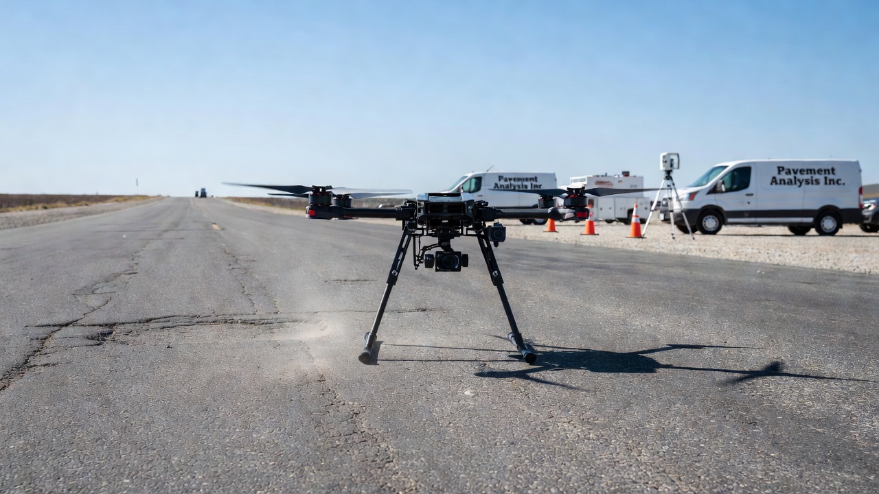
The technical workflow for UAV-based IRI estimation involves several stages. UAVs fly at altitudes of 30 to 100 meters above the pavement surface, capturing overlapping images with forward overlap ≥ 80% and side overlap ≥ 60% to ensure robust 3D reconstruction. For photogrammetry-based approaches, a camera with a mechanical shutter and a high-resolution sensor (≥ 20 megapixels) is used to avoid rolling shutter distortion and ensure adequate ground sampling distance (GSD) — typically ≤ 2 mm per pixel to resolve the profile wavelengths relevant to IRI. For LiDAR-based approaches, a UAV-mounted laser scanner with ≥ 200,000 points per second and range accuracy ≤ 10 mm is used to directly capture the 3D surface geometry.
The captured imagery or point cloud data is processed using Structure from Motion (SfM) photogrammetry software (for images) or direct point cloud filtering and classification algorithms (for LiDAR). Ground Control Points (GCPs) surveyed with RTK-GPS are essential to achieve absolute vertical accuracy of ≤ 5 mm, which is necessary for meaningful IRI computation. The resulting Digital Elevation Model (DEM) or classified point cloud is then sampled along the wheelpaths at the standard 25 mm interval to produce a synthetic longitudinal elevation profile. This profile is processed through the IRI quarter-car algorithm per ASTM E1926 to compute the estimated IRI.
Research studies comparing UAV-derived IRI to traditional inertial profiler measurements have reported promising results. Studies published in MDPI Applied Sciences, ASCE Journal of Transportation Engineering, and Transportation Research Record have demonstrated correlation coefficients (R²) between 0.75 and 0.92 for UAV photogrammetry compared to reference inertial profiler data, with root-mean-square errors typically in the range of 0.2 to 0.4 m/km (13 to 25 in/mi). The accuracy tends to be better on smooth to moderately rough pavements (IRI < 3.0 m/km) and degrades on severely rough pavements. LiDAR-based approaches generally achieve slightly better accuracy than photogrammetry, particularly for texture-rich surfaces where photogrammetric reconstruction may smooth fine-scale features.
Key limitations of UAV-based IRI estimation remain. The method cannot match the vertical resolution of laser-based inertial profilers (±0.025 mm) — typical UAV photogrammetry achieves ±2–5 mm vertical accuracy even with GCPs, which may be insufficient for precision applications such as construction acceptance. The method is sensitive to lighting conditions (shadows, glare), surface texture (uniform asphalt surfaces provide poor photogrammetric texture), and vegetation or surface debris. Flight restrictions near airports (the very locations where runway roughness assessment is needed) may limit operational feasibility. The technique has not yet been adopted as a regulatory standard by FHWA, FAA, or AASHTO, and remains primarily a research and screening tool rather than a replacement for certified inertial profilers. However, as UAV sensor technology improves and as machine learning methods for profile reconstruction advance, drone-based IRI is likely to become an accepted supplementary method within the next decade.
IRI data occupies a central position in modern Pavement Management Systems (PMS) — the systematic frameworks that transportation agencies use to monitor pavement condition, predict future deterioration, evaluate treatment alternatives, and allocate limited maintenance and rehabilitation budgets. Within PMS, IRI serves multiple distinct functions: as a performance measure for condition assessment and reporting, as a trigger for maintenance and rehabilitation decisions, as a prediction variable in deterioration models, and as an outcome metric for evaluating treatment effectiveness.
At the network level, IRI is the most commonly reported pavement condition metric because it is objective, instrument-based, and directly related to the user experience. Agencies such as state DOTs survey their entire network — typically on a 1- to 2-year cycle for Interstate and NHS routes and a 2- to 4-year cycle for lower functional classes — using high-speed inertial profilers. The resulting IRI data is aggregated into condition categories (Good/Fair/Poor), analyzed for trends over time, and used to report the percentage of the network in each condition category to legislators, stakeholders, and the public. The FHWA National Performance Management Measures rule (23 CFR Part 490) requires state DOTs to establish 2- and 4-year targets for the percentage of Interstate and non-Interstate NHS pavements in Good and Poor condition based largely on IRI.
IRI thresholds serve as decision triggers within PMS treatment selection logic. When a pavement section’s IRI exceeds a critical threshold — typically 170 in/mi (2.7 m/km) for high-volume highways or 220 in/mi (3.5 m/km) for lower-volume roads — the section is flagged as a candidate for corrective action. The specific treatment triggered depends on the underlying distress mechanism. If roughness is caused by surface distresses (raveling, minor cracking) without structural deficiency, a thin overlay or surface treatment may be appropriate. If roughness is caused by structural deterioration (deep cracking, rutting, base failure), a structural overlay or full-depth reconstruction is indicated. IRI alone cannot distinguish between these cases, which is why PMS integrates IRI with distress-based indices (PCI) and structural capacity data (falling weight deflectometer) for treatment selection.
PMS relies on pavement deterioration models to predict future condition and optimize treatment timing. IRI deterioration is typically modeled using empirical regression equations — most commonly a family of curves relating IRI to age, cumulative traffic loading (ESALs), pavement structure (thickness, material type), and environmental factors (freeze index, precipitation). Common model forms include linear: IRI(t) = IRI₀ + α × t, power-law: IRI(t) = IRI₀ + α × t^β, and sigmoidal or exponential forms for pavements approaching terminal serviceability. The initial IRI (IRI₀) — the IRI immediately after construction or treatment — is a critical model parameter that strongly influences long-term performance: pavements built smoother maintain lower IRI throughout their service life, which is the basis for smoothness-based pay adjustment specifications in construction contracts.
The HDM-4 (Highway Development and Management Model), the World Bank’s pavement management economic analysis software, is the most globally recognized system integrating IRI into a comprehensive deterioration, user cost, and economic evaluation framework. HDM-4 uses IRI progression as a primary indicator of pavement deterioration and calculates vehicle operating costs (fuel, maintenance, tire wear, depreciation), travel time costs, and road user costs as functions of IRI. The model demonstrates that vehicle operating costs increase by approximately 4–8% for every 1 m/km increase in IRI, providing the economic justification for timely maintenance interventions that prevent IRI from deteriorating beyond economically optimal trigger points.
After a pavement treatment is applied, the post-treatment IRI is measured to verify that the treatment achieved the specified smoothness target. The difference between pre-treatment and post-treatment IRI quantifies the improvement in ride quality. Pavement management systems track these outcomes to evaluate treatment effectiveness and calibrate the post-treatment IRI₀ used in deterioration models. Performance-based specifications link contractor payment to achieved IRI — contractors receive bonuses for exceeding minimum smoothness requirements and penalties or required corrective action for failing to meet them. Typical smoothness pay adjustment schedules provide a bonus of 1–5% of the bid price for each 10 in/mi of improvement below the specification threshold, with penalties of equivalent magnitude for exceeding the threshold.
At the strategic level, IRI trends inform Transportation Asset Management Plans (TAMPs) required under federal regulations. These plans establish long-term (10-year) performance targets and funding scenarios to maintain or improve network condition. IRI serves as the primary outcome indicator for ride quality investments. Scenario analyses in TAMPs use IRI predictions to compare the impacts of different funding levels — for example, a “preservation-first” strategy that applies preventive treatments before IRI reaches a critical threshold is typically more cost-effective than a “worst-first” strategy that addresses only failed pavements, as measured by the total vehicle operating cost savings per dollar of agency expenditure.
Because IRI was designed as a universal reference scale, conversion equations exist to relate IRI to legacy roughness measures. These conversions are approximate and depend on the measurement methodology of the legacy index, but they are essential for agencies comparing current IRI data to historical records.
| Legacy Index | Conversion to IRI (m/km) | Source |
|---|---|---|
| PSI (Paterson) | IRI = −5.5 × ln(PSI/5) | World Bank, 1986 |
| Profile Index (California) | IRI ≈ PI × 0.028–0.038 | State-specific calibration |
| Mays Ride Number | IRI ≈ 0.4 + 0.008 × (100−MRN) | Equipment-dependent |
| NAASRA Roughness Meter | IRI ≈ NRM × 0.38 | Australian Road Research Board |
| Quarter-Car Index (QI) | IRI = QI | Essentially identical for standard speeds |
The Profile Index (PI) — commonly expressed in mm/km from California-type profilograph traces — requires calibration to IRI because different profilograph configurations (blanking band width, wheelbase) produce different PI values for the same profile. The typical conversion is PI × 0.035, but the exact factor should be determined through local calibration on reference profiles.
For response-type meters, the calibration equation is equipment-specific and must be re-established whenever the vehicle, suspension, or tires change significantly. The equation takes the general form: IRI = A + B × RTRRM_reading, where A and B are determined by regression against reference profiles. The slope coefficient B typically ranges from 0.005 to 0.02 m/km per count, and the intercept A accounts for the meter reading on a perfectly smooth surface (which may not be zero due to mechanical noise in the sensor). +++
Leverage advanced IRI measurement technologies and data-driven pavement management strategies to reduce costs and extend asset life.
A vehicle-mounted inertial profiler uses laser height sensors and accelerometers to measure longitudinal pavement profile at highway speeds, computing IRI and r...
A profilograph is a low-speed rolling straightedge device that measures longitudinal pavement profile deviations to assess smoothness. California and Rainhart p...
ASTM D6433-20 defines the Pavement Condition Index (PCI) methodology for roads and parking lots, establishing inspection unit definition, distress identificatio...