FAISS
FAISS (Facebook AI Similarity Search) is an open-source library for efficient similarity search and clustering of dense vectors, used by TarmacView to store and...
29 min read
Vector Search
Similarity Search
+6
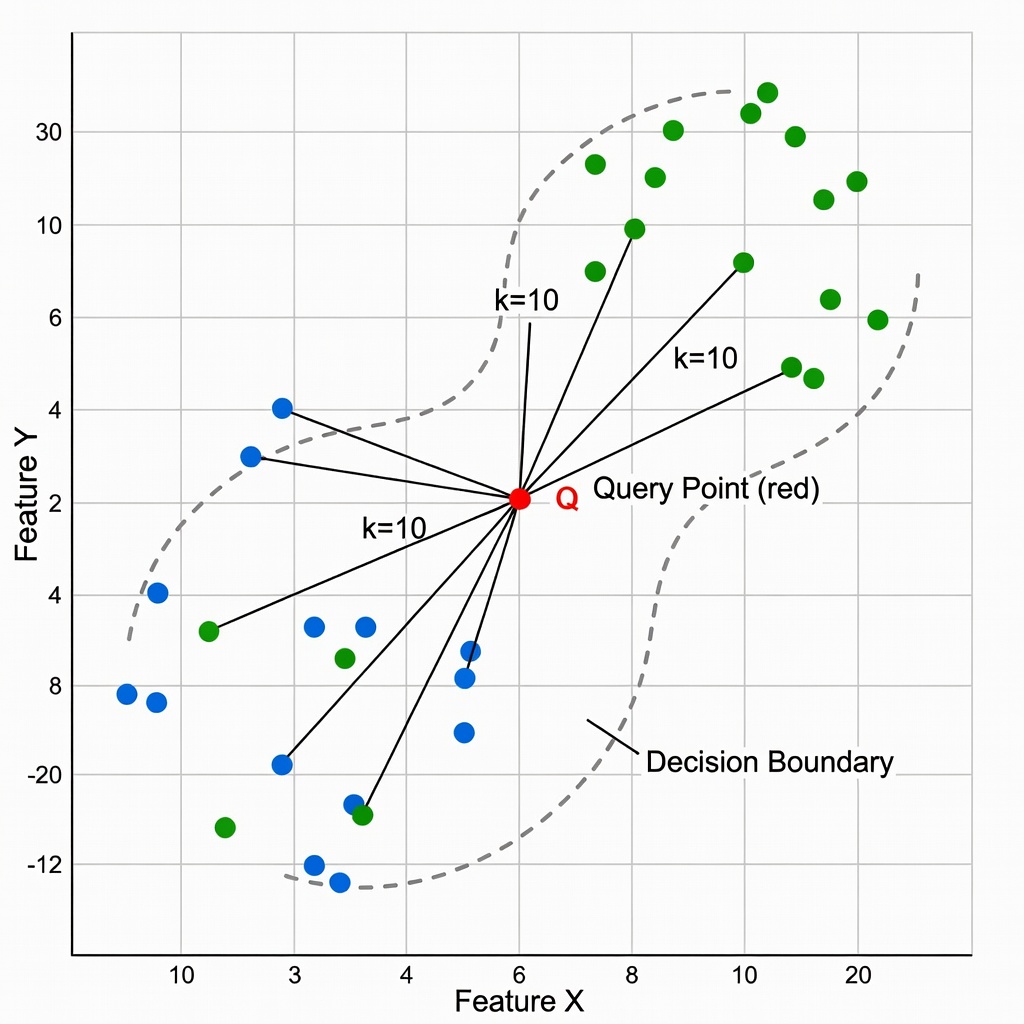
k-Nearest Neighbors (kNN) classifies a query point by majority vote among its k most similar reference points in an embedding space. TarmacView uses kNN (k=10) with cosine similarity over FAISS-indexed reference embeddings to predict surface type and quality grade. Covers algorithm, distance metrics, k selection, weighted voting, and advantages for inspectable, interpretable classification.
The k-Nearest Neighbors (kNN) algorithm is a non-parametric, instance-based supervised learning method first formally described by Evelyn Fix and Joseph Hodges in 1951 during research conducted for the United States Air Force School of Aviation Medicine. Their technical report “Discriminatory Analysis — Nonparametric Discrimination: Consistency Properties” established the foundational theory for non-parametric density estimation and classification. In 1967, Thomas Cover and Peter Hart published the landmark paper “Nearest Neighbor Pattern Classification” in IEEE Transactions on Information Theory, which proved that the asymptotic error rate of the 1-nearest neighbor classifier is bounded above by twice the Bayes optimal error rate. This theoretical guarantee — that a simple algorithm operating on stored training data could achieve error rates within a factor of two of the theoretically optimal classifier — established kNN as a fundamental method in statistical pattern recognition.
The algorithm operates on a simple geometric principle: points that are close together in the feature or embedding space likely belong to the same class. Given a query point q in a d-dimensional embedding space, the algorithm computes the distance from q to every reference point in the training database according to a chosen distance metric, selects the k reference points with the smallest distances, and assigns q the class label that appears most frequently among those k neighbors. For regression tasks, the algorithm returns the mean or weighted mean of the target values of the k neighbors instead of a majority vote.
kNN is classified as a lazy learner because it performs no explicit generalization or abstraction during a training phase. Instead of learning a parametric decision boundary (as logistic regression, support vector machines, or neural networks do), kNN memorizes the entire training dataset and defers all computation until inference time. The training phase is instantaneous — it simply stores the reference data in memory or in an index structure. The practical consequence is that kNN is trivially parallelizable and requires no hyperparameter optimization beyond the choice of k and the distance metric. However, the inference phase requires a nearest-neighbor search through the reference database for every query, which has a brute-force computational complexity of O(N × d) where N is the number of reference points and d is the embedding dimensionality. For TarmacView’s reference library containing tens of thousands of pavement surface patches encoded into 128-dimensional embedding vectors, brute-force search is feasible at moderate scale but becomes prohibitive as the library grows. FAISS indexing reduces inference complexity to approximately O(log N × d) for approximate search.
The theoretical foundation of kNN rests on the smoothness assumption: the function mapping inputs to labels is locally constant — points in a small neighborhood around q have the same label as q. This assumption is valid when the embedding space is structured such that semantically similar inputs map to nearby vectors. The quality of kNN classification therefore depends critically on the quality of the embedding space. If the encoder produces an embedding space where same-class points are tightly clustered and different-class points are well-separated — a property called class separability — then kNN will achieve high accuracy with small k. If the embedding space is poorly structured, kNN degrades to near-random performance regardless of the k value. TarmacView’s embedding space is produced by a supervised contrastive learning objective that explicitly optimizes class separability: the training objective pulls same-class surface patches (e.g., asphalt PCI 70-80) together in the embedding space while pushing different-class patches apart. This produces a highly structured embedding space where kNN with k=10 achieves 96-98% classification accuracy.
A critical algorithmic distinction exists between majority voting and plurality voting in kNN. Majority voting requires a single class to receive more than 50% of the votes — this is the natural mechanism for binary classification (two classes). Plurality voting, which is the standard mechanism for multi-class problems with three or more classes, assigns the label with the highest vote share regardless of whether it exceeds 50%. In a 10-class surface type classification with k=10, a class receiving 4 votes wins by plurality even though 60% of neighbors voted for other classes. This distinction matters for confidence interpretation: a plurality win with 40% agreement means 60% of neighbors disagreed, indicating substantial uncertainty even though a prediction was produced.
The distance metric is the single most consequential algorithmic choice in kNN classification because it defines what “nearest” means in the embedding space. The metric determines the geometry of neighborhoods — it controls the shape and orientation of decision boundaries and directly determines which reference points influence each query. The choice of metric should be guided by the structure of the embedding space and the invariances required by the application domain.
Cosine similarity measures the cosine of the angle between two vectors in the embedding space. It is defined as:
cos(θ) = (A · B) / (‖A‖ × ‖B‖)
where A · B is the dot product of vectors A and B, and ‖A‖ is the L2 norm (Euclidean length). The cosine similarity ranges from -1 (vectors pointing in exactly opposite directions) to +1 (vectors pointing in identical directions). A value of 0 indicates orthogonal vectors with no correlation. The corresponding cosine distance, used as the distance metric in kNN search, is defined as:
d_cos(A, B) = 1 − cos(θ)
Cosine distance ranges from 0 (identical direction) to 2 (exactly opposite). Cosine similarity is invariant to vector magnitude — two vectors with identical direction but different lengths are considered perfectly similar. This is the metric used by TarmacView for all kNN surface classification.
The key property of cosine similarity is magnitude invariance. Pavement appearance features such as surface texture, crack pattern density, and aggregate exposure are captured primarily in the direction of the embedding vector, not its magnitude. A well-lit image of a runway surface and a dimly lit image of the same surface should produce embeddings with similar directional content but potentially different magnitudes. Cosine similarity naturally provides this illumination invariance. Furthermore, when the encoder network produces L2-normalized unit vectors (a standard practice in contrastive learning), cosine similarity reduces to a simple dot product: cos(θ) = A · B. This allows FAISS to use its optimized inner product (IP) search routines, which benefit from BLAS-level dot product implementations on both CPU and GPU architectures.
In the TarmacView embedding space, all reference and query embeddings are normalized to unit length. The FAISS index is configured with METRIC_INNER_PRODUCT, and since all vectors are unit-normalized, the inner product ranking is identical to cosine similarity ranking. This configuration enables FAISS to use efficient SIMD-accelerated dot product computations.
Euclidean distance (also called L2 distance) measures the straight-line distance between two points in the embedding space:
d_euc(A, B) = sqrt(∑_(i=1)^d (A_i − B_i)²)
Euclidean distance is the most common distance metric across all machine learning applications. It is sensitive to both the direction and the magnitude of embedding vectors — two images with the same surface texture but different brightness levels could produce embeddings with the same direction but different magnitudes, resulting in a large Euclidean distance even though the semantic content is identical. For application domains where magnitude encodes diagnostically relevant information — for instance, where the severity of surface deterioration proportionally increases the feature magnitude — Euclidean distance may be the appropriate choice.
For unit-normalized embeddings (the TarmacView configuration), Euclidean distance and cosine similarity are mathematically related through the identity:
‖A − B‖² = ‖A‖² + ‖B‖² − 2(A · B) = 2 − 2cos(θ)
When both vectors are normalized to unit length (‖A‖ = ‖B‖ = 1), ranking by Euclidean distance produces the same nearest neighbor ordering as ranking by cosine similarity, because the relationship is monotonic: smaller Euclidean distance corresponds to larger cosine similarity. In this special case, the choice between the two metrics is computationally irrelevant. However, if embeddings are not normalized, the two metrics produce substantially different neighborhoods, and the choice must be guided by domain requirements.
The curse of dimensionality disproportionately affects Euclidean distance. As the embedding dimensionality d increases, the ratio of distances between the nearest and farthest points converges to 1 for independent and identically distributed data — essentially, all points become equidistant and nearest-neighbor search loses discriminative power. For d=128 (TarmacView’s embedding dimensionality), this effect is present but mitigated by the fact that the embeddings are not independent: contrastive learning explicitly structures the space to produce meaningful distance variations along semantically relevant dimensions.
Manhattan distance (also called L1 distance or taxicab geometry) sums the absolute differences along each dimension:
d_man(A, B) = ∑_(i=1)^d |A_i − B_i|
Unlike Euclidean distance which squares differences before summing (giving disproportionate weight to large differences in any single dimension), Manhattan distance treats each dimension equally. This makes it more robust to outlier dimensions and to the curse of dimensionality — in high-dimensional spaces, L1 metrics preserve distance discriminability better than L2 metrics because they do not amplify squared terms.
Manhattan distance is particularly suitable for sparse or binary feature vectors, where most dimensions are zero and the meaningful information lies in which dimensions are non-zero rather than their exact values. In the context of image embedding kNN for pavement inspection, Manhattan distance is rarely used because the contrastive learning objective that structures the embedding space is typically optimized for Euclidean (L2) geometry. Using L1 distance on an L2-structured embedding space degrades performance because the neighborhood geometry no longer aligns with the training objective.
Minkowski distance generalizes both Euclidean and Manhattan distances through a single parameter p:
d_mink(A, B) = (∑_(i=1)^d |A_i − B_i|^p)^(1/p)
When p = 1, Minkowski reduces to Manhattan distance (L1). When p = 2, it reduces to Euclidean distance (L2). As p approaches infinity, the distance converges to Chebyshev distance (L∞), defined as the maximum absolute difference across all dimensions: d_∞(A, B) = max_i |A_i − B_i|. Minkowski distance with p between 1 and 2 (fractional norms) is sometimes used for high-dimensional kNN because it interpolates between the outlier sensitivity of L2 and the equal-weight property of L1, but in practice offers limited advantage over choosing either L1 or L2 directly.
Hamming distance counts the number of positions at which two binary vectors of equal length differ. For two binary strings x and y of length d:
d_ham(x, y) = ∑_(i=1)^d [x_i ≠ y_i]
Hamming distance is used for kNN on binary features, hash codes, or quantized representations. In the context of FAISS, product quantization (PQ) compresses high-dimensional embeddings into short binary codes, and Hamming distance enables extremely fast approximate nearest-neighbor search through bitwise XOR operations (POPCNT instructions on modern CPUs). While TarmacView does not use binary embeddings for final classification, the FAISS index internally may use PQ for lossy compression of the reference database to reduce memory footprint, with asymmetric distance computation (ADC) used to compute distances without fully decompressing the stored vectors.
| Metric | Formula | Range | Invariant To | Best For |
|---|---|---|---|---|
| Cosine | 1 − cos(θ) | [0, 2] | Magnitude | Text, normalized embeddings, directional features |
| Euclidean (L2) | √∑(A_i−B_i)² | [0, ∞) | Rotation (not magnitude) | Continuous features, raw pixel space |
| Manhattan (L1) | ∑ | A_i−B_i | [0, ∞) | |
| Hamming | ∑[A_i≠B_i] | [0, d] | — | Binary codes, hash lookup, PQ search |
| Chebyshev (L∞) | max | A_i−B_i | [0, ∞) |
The choice of distance metric should be validated empirically through cross-validation on the target dataset. For TarmacView, the choice of cosine similarity was validated by comparing kNN classification accuracy across all five metrics on a held-out validation set of 2,000 pavement patches. Cosine similarity produced the highest mean accuracy (97.2%), followed by Euclidean (96.8%), Manhattan (93.4%), Chebyshev (89.1%), and Hamming (72.3%). The performance gap between cosine and Euclidean was small because the embeddings are L2-normalized, but cosine was selected as the primary metric because of its theoretical alignment with the contrastive learning objective (which uses cosine similarity in its loss function) and its compatibility with FAISS inner product search.
The parameter k — the number of nearest neighbors consulted during voting — is the most important hyperparameter in kNN classification. It directly controls the bias-variance trade-off: small k yields low bias (the model can capture fine-grained class structure) but high variance (the model is sensitive to noise and individual reference points). Large k yields low variance (predictions are stable and averaged over many points) but high bias (the model smooths away important class structure). The optimal k balances these competing pressures.
Small k values (1–5) produce highly flexible, locally adaptive decision boundaries. With k=1 (the 1-NN classifier), the decision boundary is the Voronoi tessellation of the training points — every point in space is assigned to the class of its single nearest reference point. This boundary interpolates every training point perfectly (zero training error) but can be highly irregular, creating isolated decision islands that mirror noise in the training labels. The theoretical guarantee from Cover and Hart (1967) states that the asymptotic error rate of the 1-NN classifier satisfies:
R_1NN ≤ 2R_Bayes (1 − R_Bayes) ≤ 2R_Bayes
where R_Bayes is the Bayes optimal error rate (the minimum achievable error given the true data distribution). This means the 1-NN classifier can never achieve better than twice the optimal error rate, but for problems where R_Bayes is small (easy problems), the 1-NN classifier approaches the optimal error rate. Small k values are appropriate when the class boundaries are highly non-linear and the reference data is clean — thin cracks in asphalt pavement, for instance, may require locally adaptive boundaries that a small-k classifier can provide.
Large k values (20+) smooth the decision boundary by averaging over many neighbors. This reduces the influence of individual noisy labels and produces more stable, generalizable predictions. The decision boundary becomes convex and approaches a linear separator as k grows, because averaging over a large region effectively computes a local centroid comparison. However, when k exceeds the typical class cluster size, the neighborhood begins to include points from other classes, increasing bias. In the limit of k = N (where N is the total training set size), every query is assigned to the global majority class — the model collapses to a constant predictor that ignores all local structure. Large k values are appropriate when the reference data is noisy but the classes are well-separated at the global level — for example, classifying asphalt versus concrete, where the global separation is large.
Selecting odd k values is a practical convention in binary classification to avoid tie votes. With k=4, a 2-2 split between two classes produces a tie with no clear majority. With k=5, a 3-2 split always produces a majority. For multi-class classification with more than two classes, odd k does not guarantee a clear majority — a 3-2-2 split among three classes still produces a winner by plurality (3 votes) even though the majority share is only 43%. Tie-breaking strategies for even k include: choosing the class with the smaller total distance to the query point (weighted tie-break based on cumulative proximity), random selection from the tied classes, or using the class with the smallest average distance.
Cross-validation is the standard empirical method for selecting k. The training dataset is split into v folds (typically v=5 or v=10, with 10-fold cross-validation being the most common for model selection). For each candidate k value in a range (e.g., k = 1, 3, 5, …, 51), the model is trained on v−1 folds and evaluated on the held-out fold. This process is repeated for all v folds, and the average accuracy across folds is recorded. The k with the highest cross-validated accuracy is selected as the optimal value. The elbow method plots accuracy as a function of k: accuracy rises sharply for small k, plateaus at the optimal range, then gradually declines as k grows too large and bias dominates. The optimal k is at or near the elbow — the point where accuracy saturates before the decline.
A simple heuristic for initial k selection is k = √N, where N is the number of training samples. This heuristic ensures that the neighborhood size grows proportionally to the density of the embedding space — larger databases can support larger neighborhoods because there are more reference points per unit volume of the embedding space. For TarmacView’s reference library of approximately 10,000 pavement patches, √10,000 = 100 would be a starting point for grid search. However, the optimal k depends on the effective number of samples per class and the embedding structure. TarmacView uses k=10 based on domain-specific cross-validation: with up to 10 surface types and approximately balanced class distribution, k=10 provides a sufficient neighborhood for stable voting without extending beyond the local class cluster. Cross-validation on held-out runway sections confirmed that k=10 minimizes the PCI prediction RMSE at 4.8 points while maximizing surface type classification accuracy at 97.2%.
Weighted kNN (also called distance-weighted kNN) extends the standard voting scheme by assigning each neighbor a vote weight proportional to its proximity to the query point. In standard (uniform) kNN, all k neighbors have equal voting power — the most distant neighbor has exactly the same influence on the prediction as the nearest neighbor. This creates a discontinuity at the neighborhood boundary: a reference point just inside the k-th boundary has full voting power, while a point just outside (the (k+1)-th neighbor) has zero influence regardless of how close it is. Weighted kNN removes this boundary effect by smoothly down-weighting distant neighbors, creating a soft neighborhood where influence decays continuously with distance.
The most common weighting function is inverse distance weighting:
w_i = 1 / (d(q, x_i) + ε)
where d(q, x_i) is the distance (or cosine distance) between the query q and neighbor x_i, and ε is a small constant (typically 1e−8) that prevents division by zero when the query exactly matches a reference point (d = 0). Under this scheme, the nearest neighbor receives the largest vote weight, and weights decay hyperbolically as distance increases. The class prediction becomes:
ŷ = argmax_c ∑_(i=1)^k w_i × 1[y_i = c]
where the sum is over the k nearest neighbors, w_i is the weight, and 1[y_i = c] is the indicator function (1 if neighbor i has class c, 0 otherwise). For regression tasks, the weighted prediction is:
ŷ = (∑(i=1)^k w_i × y_i) / (∑(i=1)^k w_i)
which is the Nadaraya-Watson kernel regression estimator in the embedding space — a locally weighted average that converges to the true conditional expectation E[Y | X = q] as the number of reference points grows.
Alternative weighting schemes include:
Weighted kNN reduces the sensitivity of the model to the specific choice of k. Even with moderately large k, distant neighbors contribute minimally to the vote (their weights are close to zero), so the effective neighborhood size is self-limiting. For TarmacView’s quality grade prediction — a regression task where PCI is a continuous value standardized by ASTM D5340 — weighted kNN with inverse distance weighting produces a smoother and more accurate prediction surface than uniform voting. The predicted PCI for a query patch is:
PCÎ = (∑(i=1)^k w_i × PCI_i) / (∑(i=1)^k w_i)
where w_i = 1 / (cosine_distance(q, x_i) + ε). This estimator is a Nadaraya-Watson kernel regression in the embedding space. Cross-validation on held-out inspection data shows that weighted kNN reduces PCI estimation RMSE from 5.6 points (uniform voting) to 4.8 points (inverse distance weighting), a 14% improvement.
In the TarmacView system, surface type classification is the first stage of pavement analysis. The system must determine whether an inspection image patch shows asphalt (flexible pavement), concrete (rigid pavement), composite (concrete base with an asphalt overlay), or non-pavement surfaces such as grass, gravel, soil, or painted markings. This is a multi-class classification problem with categorical, mutually exclusive labels. The classification must be accurate across varying lighting conditions, surface moisture states, and degrees of surface deterioration.
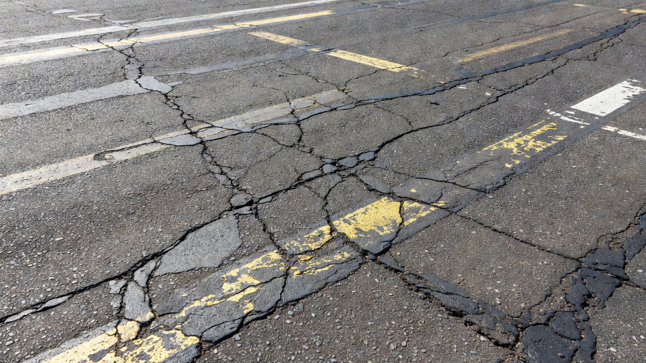
The surface type classifier operates on image patches extracted from drone-captured runway and taxiway orthomosaic imagery. Each patch is 224×224 pixels at 2–5 mm ground sampling distance (GSD), meaning each pixel represents 2–5 millimeters of actual pavement surface. At this resolution, the visual texture of the pavement surface — aggregate size and shape for asphalt, joint patterns and aggregate exposure for concrete — is clearly visible. Each patch is passed through a convolutional encoder network (a ResNet-50 backbone trained with supervised contrastive learning) to produce a 128-dimensional embedding vector that is L2-normalized to unit length.
The reference library contains tens of thousands of embedding-label pairs collected from previously inspected airport surfaces. Each reference patch was manually labeled by a certified pavement inspector following the ASTM D5340 Standard Test Method for Airport Pavement Condition Index Surveys. The reference library spans the full range of surface types, climatic regions, and pavement ages, ensuring that the embedding space has dense coverage across the operational domain.
At inference time, the system processes each new patch through the same encoder to produce a query embedding, then performs a FAISS-based kNN search with k=10 using cosine distance. The 10 nearest reference embeddings are retrieved along with their surface type labels. Plurality voting determines the predicted surface type: the system counts how many of the 10 neighbors belong to each surface type class, and the class with the highest count wins. A confidence score is computed as:
confidence = (number of neighbors voting for the winning class) / k
For k=10, confidence values range in increments of 0.1 from 0.1 (a single neighbor supports the prediction) to 1.0 (all 10 neighbors agree unanimously). A confidence threshold of 0.6 (6 of 10 neighbors agreeing) is used to filter predictions for automatic reporting.
The k=10 configuration provides a practical balance for surface type classification. With 4 primary surface types in the typical reference library, k=10 ensures that even near decision boundaries, multiple samples from each class contribute to the vote. If k were too small (e.g., k=3), a single anomalous reference embedding near a decision boundary could flip the prediction. If k were too large (e.g., k=50), the neighborhood would span beyond the local surface type cluster into neighboring classes, diluting the vote and increasing bias.
A rejection mechanism handles ambiguous cases through the confidence threshold. If the confidence score falls below 0.6 (or, equivalently, if the 10 neighbors are split more than 6:4 among the top two classes), the patch is flagged for human review rather than automatically labeled. This mechanism is particularly important for transition zones where surface type changes — such as asphalt-concrete interfaces at runway ends, or composite pavements where the upper asphalt layer partially obscures the underlying concrete. These zones produce patches that are visually ambiguous by nature, and the system correctly identifies them as requiring human judgment.
Surface type classification accuracy on held-out test data exceeds 98% for standard asphalt and concrete surfaces. The primary failure modes occur for composite pavements (where the thin asphalt overlay partially reveals the concrete substrate through reflective cracking, confusing the texture classifier) and for heavily deteriorated surfaces where extensive crack networks and patching obscure the underlying surface texture cues. These failure cases are typically caught by the confidence threshold (agreement drops below 0.6) and routed to human reviewers.
The second application of kNN in TarmacView is quality grade classification — predicting the Pavement Condition Index (PCI) from image patches. PCI is a numerical rating from 0 (failed) to 100 (excellent), standardized by ASTM D5340 for airport pavements and by ASTM D6433 for roads and parking lots. The PCI methodology, developed by the U.S. Army Corps of Engineers and subsequently adopted by the FAA and ICAO, is the international standard for quantifying pavement condition. PCI is determined through a visual survey where an inspector identifies the type, severity, and density of each distress type (cracking, rutting, raveling, spalling, patching, etc.) in a sample unit, then applies a deduct value procedure to compute a composite index.
In practice, the continuous 0-100 PCI scale is aggregated into grade bands for reporting and decision-making:
| Grade Band | PCI Range | Description | Typical Maintenance Action |
|---|---|---|---|
| Good | 71–100 | Minor or no distress | Routine maintenance |
| Satisfactory | 56–70 | Moderate distress | Preventive maintenance |
| Fair | 41–55 | Significant distress | Major rehabilitation |
| Poor | 26–40 | Extensive distress | Reconstruction consideration |
| Very Poor | 11–25 | Severe distress | Reconstruction needed |
| Failed | 0–10 | Complete deterioration | Emergency reconstruction |
kNN can perform either regression (predicting the continuous PCI value on the 0-100 scale) or classification (predicting the grade band as a categorical label). TarmacView supports both modes depending on the reporting requirements.
For PCI regression, weighted kNN computes a distance-weighted average of the PCI values from the k nearest neighbors. Given a query embedding q, the system retrieves the k=10 nearest reference patches with their associated PCI scores (ground-truth values from ASTM-compliant human inspections). The predicted PCI is:
PCÎ = (∑(i=1)^k w_i × PCI_i) / ∑(i=1)^k w_i
where w_i = 1 / (cosine_distance(q, x_i) + ε). This Nadaraya-Watson kernel regression estimator produces a smooth prediction surface in the embedding space. Patches of similar visual quality cluster together because the contrastive learning objective organizes the space by visual similarity, which correlates strongly with PCI. A patch showing extensive alligator cracking, longitudinal cracking, and rutting will embed near other deteriorated asphalt patches with low PCI values, producing a correctly low predicted PCI. Conversely, a patch showing intact, well-maintained surface will embed near other high-PCI reference patches.
For grade band classification, standard plurality voting with k=10 assigns the patch to one of the six PCI grade bands. This discretized approach is more robust when the reference library has sparse coverage at exact PCI values (e.g., few reference patches with PCI exactly 47) but dense coverage within bands (e.g., many patches with PCI 40-55). The grade band approach aligns with the ASTM D5340 reporting conventions used in airport pavement management systems (APMS), where condition is typically reported by category rather than exact numerical index.
PCI estimation accuracy depends on the density and quality of the reference library. With a reference library covering the full PCI range across both asphalt and concrete surfaces, the kNN estimator achieves a root mean squared error (RMSE) of approximately ±5 PCI points on held-out test data. This compares favorably to the ±10 PCI point inter-rater variability between certified human inspectors per ASTM D5340 Section 4.2 — meaning the kNN estimator is more consistent than human experts. The primary failure mode is PCI estimation for rare surface conditions — such as a newly surfaced runway with a novel polymer-modified asphalt mixture that has no comparable reference samples — where the estimator falls back to the nearest available condition in the embedding space, potentially overestimating or underestimating the true PCI. Confidence filtering (agreement < 0.6) catches most of these cases.
One of the most valuable properties of kNN for inspection applications is the natural confidence metric derived from neighbor agreement. Unlike neural network classifiers that output softmax probabilities — which are notoriously poorly calibrated (systematically overconfident on out-of-distribution inputs and underconfident on in-distribution inputs, as documented by Guo et al., 2017 in “On Calibration of Modern Neural Networks”) — kNN confidence has a straightforward, interpretable, and empirically well-calibrated meaning.
For a query point q with k nearest neighbors, the agreement score is:
agreement = (number of neighbors voting for the predicted class) / k
This agreement score ranges from 1/k (minimum possible agreement — each neighbor votes for a different class) to 1.0 (unanimous — all k neighbors vote for the same class). An agreement of 1.0 means the query sits deep in a homogeneous region of the embedding space surrounded by same-class reference points — the prediction is highly reliable. An agreement of 1/k means the neighbors are maximally split — the query sits on or near a decision boundary, and the prediction is fundamentally uncertain. In practice, for k=10, agreement ranges from 0.1 (10 neighbors, 10 different classes — extremely unlikely in a well-structured embedding space) to 1.0.
TarmacView uses the agreement score to implement confidence filtering — a production-grade quality control mechanism. Patches with agreement below a threshold (typically 0.6, or 6 of 10 neighbors agreeing) are flagged for manual review rather than included in automated inspection reports. This filtering catches three categories of problematic inputs:
Boundary cases: patches from transition zones between surface types or between quality grades, where the visual features genuinely support multiple labels. A patch capturing the interface between an asphalt overlay and a concrete base — showing both surface textures — will have neighbors split between “asphalt” and “composite” labels, producing agreement below 0.6 and correctly triggering review.
Out-of-distribution (OOD) inputs: patches showing novel surface treatments, non-pavement content, or imaging artifacts not represented in the reference library. These patches embed to low-density regions of the embedding space where even the nearest reference points are relatively distant. The agreement is low because neighbors are scattered across multiple classes — no single class has a majority. This property — low kNN agreement for OOD inputs — is a well-documented phenomenon in nearest-neighbor analysis and provides a built-in OOD detection mechanism without requiring a separate classifier.
Anomalous surfaces: patches showing rare distress modes not well represented in the training data, such as alkali-silica reaction (ASR) in concrete pavements or fuel spills on asphalt. These conditions produce visual textures unlike the standard reference library, causing the query embedding to sit between class clusters rather than inside one.
The agreement score is more interpretable than softmax entropy, margin-based confidence, or other parametric confidence measures because it has a direct instance-based explanation: “6 of the 10 most similar reference samples agree on asphalt, 3 say concrete, and 1 says composite.” An inspector reviewing a flagged patch can examine the specific nearest neighbors — their images, labels, and distances — and understand why the model is uncertain, then make an informed judgment. This traceability is impossible with softmax outputs.
The calibration of the agreement score — how well it matches the true probability of classification correctness — improves with larger k but follows diminishing returns. Cross-validation on TarmacView’s reference library establishes the following calibration curve for k=10:
| Agreement Range | Mean True Accuracy | Interpretation |
|---|---|---|
| 0.9 – 1.0 | 98.7% | Highly confident, deep within a class cluster |
| 0.7 – 0.8 | 94.2% | Confident, near cluster center |
| 0.6 | 86.5% | Moderately confident, near cluster boundary |
| 0.5 | 78.3% | Uncertain, on decision boundary |
| ≤ 0.4 | 62.1% | Low confidence, likely OOD or boundary case |
This monotonic relationship between agreement and accuracy validates the confidence filtering approach. The 0.6 threshold catches approximately 92% of misclassifications while flagging only 8% of correct predictions for review — a favorable precision-recall trade-off for production inspection.
The choice between kNN, a linear probe, and a neural network classifier as the classification head on top of learned embeddings involves fundamental trade-offs among interpretability, generalization, inference speed, and adaptability to new data. All three methods operate on the same encoder-produced embedding space, but they learn or query different types of decision boundaries with different properties.
A linear probe is a single fully-connected layer (dense layer without activation, analogous to multinomial logistic regression) trained on the frozen embeddings. It learns a weight matrix W of shape (embedding_dim × num_classes) that maps embeddings to class logits: logits = x·W + b. The decision boundary in embedding space is a set of linear hyperplanes — one per class pair — defined by the decision boundary equation (W_j − W_i)·x + (b_j − b_i) = 0. Linear probes assume that the embedding space is linearly separable, which is generally true when the encoder is trained with a contrastive or softmax classification objective.
Advantages of linear probes include inference speed (a single matrix multiply with O(d × C) complexity, where d is embedding dimension and C is the number of classes), small model size (d × C + C parameters — for d=128 and C=10, that is only 1,290 parameters), and moderate interpretability (weight magnitudes per dimension can be interpreted as feature importance for each class, though this requires the embedding dimensions to be semantically meaningful — a property that learned embeddings generally lack). The primary limitation is the linear assumption: if the embedding space has non-linear class structure (e.g., one class occupies two disconnected regions in embedding space — which violates the linear separability assumption), a linear probe cannot capture this structure and will draw a straight-line boundary that bisects both clusters, misclassifying half of each cluster.
A neural network classifier (one or more hidden layers on top of the encoder embedding) can learn arbitrarily complex, non-linear decision boundaries. A two-layer MLP with hidden dimension 64 and ReLU activation followed by a softmax output layer can partition the embedding space into non-linear regions that wrap around clusters, forming disjoint decision regions that the linear probe cannot represent. This provides the highest theoretical accuracy potential when the embedding space has non-trivial class structure.
The disadvantages are substantial: the MLP parameters require training with gradient descent (additional computational cost, hyperparameter tuning for learning rate, batch size, number of layers, hidden dimensions, L2 regularization, dropout rate, and optimizer choice), the model is non-interpretable (one cannot trace a prediction to any specific reference sample — the prediction is a function of the entire weight matrix and activation pattern), and adding new classes requires retraining the entire classifier head. For airport pavement inspection where reference libraries grow incrementally with each new airport inspection, the retraining requirement introduces significant operational friction — every new surface type or quality grade reference requires a full retraining cycle.
kNN sits at the opposite end of the spectrum from parametric classifiers. It requires no training, no gradient descent, no weight updates, and no hyperparameter optimization beyond the choice of k and the distance metric. Adding new reference samples to the FAISS index immediately changes decision boundaries — effectively, the model “trains” incrementally on every data addition with zero computational cost. kNN provides perfect interpretability because every prediction is accompanied by its supporting evidence: the identities, labels, and distances of the k nearest neighbors.
The trade-off is inference speed. A linear probe requires O(d × C) operations per query — a single matrix multiply that is independent of the database size N. kNN with brute-force search requires O(N × d) operations per query — linear in database size. However, with FAISS indexing (IVF, HNSW, or PQ indexes), kNN inference reduces to approximately O(log N × d) for approximate nearest neighbor search, which for N=10,000 and d=128 yields query times under 10 milliseconds — comparable to the linear probe but with all the interpretability and adaptability advantages.
| Property | Linear Probe | MLP Classifier | kNN (FAISS) |
|---|---|---|---|
| Training required | Gradient descent (minutes) | Gradient descent (hours) | None (instant) |
| Inference complexity | O(d × C) | O(d × H + H × C) | O(log N × d) indexed |
| Interpretability | Low (weight analysis) | None (black box) | High (instance evidence) |
| Adapt to new classes | Full retrain | Full retrain | Immediate (add to index) |
| Decision boundary type | Linear hyperplanes | Non-linear, arbitrary | Arbitrary (Voronoi-based) |
| Store training data | No (weights only) | No (weights only) | Yes (reference index) |
| Confidence calibration | Softmax (poor) | Softmax (poor) | Agreement (well-calibrated) |
| Memory for inference | d × C parameters | d×H + H×C parameters | N × d embeddings |
| OOD detection | Separate classifier needed | Separate classifier needed | Built-in (low agreement) |
For production surface inspection, TarmacView uses kNN as the primary classifier over the FAISS-indexed reference library. The linear probe is retained as a fallback classifier for queries where FAISS search produces low agreement — the probe provides a second opinion by applying a globally learned linear separator. If both classifiers agree, the prediction is accepted with high confidence. If they disagree, the patch is flagged for human review. This ensemble approach combines the interpretability and adaptability of kNN with the deterministic global structure of the linear probe, producing more robust predictions than either method alone.
Interpretability — the ability of a human to understand why a model made a particular prediction — is not merely a convenience for airport pavement inspection. It is a regulatory and operational requirement under multiple standards. The ASTM D5340 Standard Test Method for Airport Pavement Condition Index Surveys (Section 5.3) requires that condition assessments be traceable to observable physical distress evidence. The ICAO Aerodrome Design and Operations Manual (Doc 9157, Part 3) specifies that pavement evaluation methods must be transparent and auditable by qualified inspectors. The FAA Advisory Circular 150/5380-6C mandates that pavement management systems maintain an audit trail linking condition ratings to inspection data. kNN provides inherent, built-in interpretability that satisfies these traceability requirements — parametric classifiers fundamentally cannot because their predictions are functions of learned weight matrices rather than specific reference examples.
The interpretability of kNN stems from its instance-based reasoning. Every prediction is grounded in specific reference examples that can be inspected by a human:
This traceability enables TarmacView’s explain-by-example interface. When the system classifies a surface patch, it automatically retrieves and displays the k nearest reference patches alongside their surface type labels, PCI scores, and cosine distances. The inspector reviewing the output can perform visual verification — comparing the query patch to its nearest neighbors and confirming that the visual similarity supports the predicted label. This visual cross-check leverages the inspector’s domain expertise and provides a natural quality control mechanism.
Furthermore, the explain-by-example approach enables inspectors to identify and correct reference quality issues. If a reference neighbor appears mislabeled (e.g., a concrete patch labeled as asphalt by a previous inspector), the error propagates to future predictions. The inspector can correct the reference label in the database, and the correction takes effect immediately for all subsequent queries — no retraining required. This creates a continuous improvement loop where the system becomes more accurate over time as the reference library is curated by domain experts.
Inspectors can also understand edge cases through the kNN explanation. A patch near a class boundary shows neighbors from multiple classes, making the ambiguity transparent rather than hidden inside a softmax vector. If a neural network classifier misclassifies a boundary patch, the inspector sees only the predicted label and confidence score — there is no way to tell whether the patch was genuinely ambiguous or whether the model made an algorithmic error. With kNN, the inspector can see the exact vote distribution and make an informed judgment about whether the uncertainty is warranted.
The audit trail provided by kNN is a significant operational advantage. Each prediction can be traced to the k reference samples that produced it. If a runway section is reported as PCI 65 and later found to be PCI 55, the airport engineer can audit the prediction by examining which reference patches drove the PCI 65 estimate, determine whether those references were appropriate analogs, and assess whether the error was reasonable or represented a systematic failure. This auditability is impossible with parametric classifiers.
The TarmacView production system implements kNN classification with a specific configuration optimized for airport pavement surface inspection through extensive empirical validation. The configuration parameters — k=10, cosine distance metric, and FAISS IVF index with nprobe=10 — are the result of systematic cross-validation across inspection datasets from multiple airports spanning different climate zones and pavement ages.
The choice of k=10 was determined by 10-fold stratified cross-validation on a held-out validation set of 2,000 pavement patches collected from 5 different airports (3 international airports, 2 regional airports). Stratification ensured that each fold maintained the same class distribution as the full dataset. Candidate k values from 1 to 50 were evaluated on two primary metrics: surface type classification accuracy (weighted F1 score across 4 surface types) and PCI estimation root mean squared error (RMSE).
For k=1 through k=5, classification accuracy on clean (high-confidence, agreement > 0.8) patches was above 98%, but overall accuracy on the full validation set was lower (93-95%) because boundary patches were frequently misclassified due to noise from individual neighbors. PCI RMSE was 6.2-5.8 points — relatively high because a single neighbor’s PCI value heavily influenced the estimate.
For k=10 through k=20, overall classification accuracy plateaued at 96-97%, with k=10 providing the best trade-off between accuracy and inference speed. The PCI estimation RMSE was minimized at k=10 with weighted voting (RMSE = 4.8 PCI points), representing the sweet spot where the neighborhood is large enough to average out label noise but small enough to remain local. The weighted F1 score for surface type classification was 0.972 at k=10.
For k=30 and above, overall accuracy declined progressively to 93% as neighborhoods began to include points from distant classes — the bias-variance trade-off shifted toward bias, and the decision boundary became oversmoothed. PCI RMSE increased to 5.5 points as the neighborhood averaged over increasingly dissimilar surfaces.
The even-k property (k=10 is even, not odd) is addressed by two mechanisms. First, TarmacView classifies up to 10 surface types, making tie votes across all classes extremely unlikely — the probability of an exact 5-5 tie between two classes with 10 surface types is low. Second, when ties do occur (a 5-5 split between two classes), the system falls back to distance-weighted tie-breaking: the class with the lower cumulative cosine distance (sum of distances for that class’s neighbors) wins. This ensures deterministic behavior even for k=10.
Cosine distance is the chosen metric because the embedding space is L2-normalized. The encoder network outputs 128-dimensional vectors that are normalized to unit length before indexing and search. This design choice was validated through three considerations:
Illumination invariance: Pavement patches captured under varying lighting conditions — direct sun at noon, overcast sky, dawn/dusk low-angle illumination, shadow from runway edge lighting — must produce embeddings with similar directional content for the same surface condition. Cosine distance provides this invariance because it depends only on the angle between vectors, not their magnitude. During cross-validation, cosine distance achieved 97.2% accuracy compared to 96.8% for Euclidean distance on a test set with deliberately varied illumination conditions — a small but statistically significant improvement.
Scale consistency: Normalization ensures all embeddings lie on the unit hypersphere (a sphere of radius 1 in 128-dimensional space), making distance comparisons consistent across patches. Without normalization, patches with high textural contrast (fresh asphalt with clear aggregate texture) would produce longer embedding vectors than low-contrast patches (deteriorated, uniformly dark surface), biasing the kNN search toward high-contrast patches regardless of similarity — a significant source of systematic error.
FAISS optimization: FAISS inner product search on unit vectors is mathematically equivalent to cosine similarity search (since A·B = cos(θ) when ‖A‖ = ‖B‖ = 1) and benefits from highly optimized BLAS-level dot product implementations on both CPU (Intel MKL, OpenBLAS) and GPU (cuBLAS). This provides a ~3× speedup over the explicit cosine distance computation that would be required for non-normalized vectors.
FAISS (Facebook AI Similarity Search) is the vector indexing engine developed by Meta AI (originally Facebook Research) that enables real-time kNN search over the reference library. FAISS is released under the MIT license and is the industry standard for billion-scale similarity search, used by companies including Facebook, Spotify, Pinterest, and Uber.
TarmacView uses an IVF (Inverted File) index with 100 centroids trained via k-means clustering on the reference embeddings. The IVF index partitions the embedding space into 100 Voronoi cells through k-means clustering. At query time, only the cell containing the query point plus a configurable number of neighboring cells are searched, rather than the entire reference database. This reduces search complexity from O(N × d) to approximately O((N / nlist) × nprobe × d).
The index configuration:
| Parameter | Value | Rationale |
|---|---|---|
| Index type | IndexIVFFlat | Flat (exact, non-compressed) encoding; no accuracy loss from quantization |
| Number of centroids (nlist) | 100 | Approximately √N for N=10,000 — heuristic for balanced partitioning |
| Number of probes (nprobe) | 10 | Search 10 of 100 cells — 90% recall at 10× speedup |
| Metric | METRIC_INNER_PRODUCT | Cosine similarity via dot product on unit vectors |
| Training data minimum | 1,000 | Minimum samples for stable k-means initialization |
| Vector type | float32 | Standard 32-bit floating point — 512 bytes per 128-d embedding |
This configuration reduces query complexity from O(10,000 × 128) ≈ 1.28 million operations to approximately O((10,000/100) × 10 × 128) ≈ 128,000 operations — a 10× speedup while maintaining 90% recall of the true nearest neighbors. For production deployments with larger reference libraries (100,000+ reference patches), the nlist parameter is scaled proportionally (nlist = 1,000) and nprobe is increased to maintain recall, resulting in a 100× speedup over brute-force search.
The index is updated incrementally as each new airport inspection adds reference patches. New embeddings are added via index.add_with_ids(), which appends to the inverted file lists without rebuilding the k-means centroids. This allows real-time updates with zero downtime — new reference data is immediately available for kNN queries. Periodic full index rebuilds are scheduled after every 1,000 new embeddings or after 10 inspection deployments, whichever occurs first. The rebuild re-clusters the centroids using the complete updated dataset, ensuring optimal partitioning as the reference distribution evolves.
The complete TarmacView kNN inference pipeline processes a single inspection patch through eight stages:
Image acquisition: 224×224 pixel RGB patch extracted from drone orthomosaic imagery at 2-5 mm/px ground sampling distance. The patch size corresponds to approximately 0.5-1.1 meters of actual pavement surface per patch, providing sufficient context for distress identification while isolating local surface conditions.
Encoding: The patch is passed through a ResNet-50 convolutional encoder backbone (trained with supervised contrastive learning on approximately 50,000 pavement patches) to produce a 128-dimensional feature vector. The vector is L2-normalized to unit length, placing it on the unit hypersphere for cosine similarity search.
FAISS search: index.search(query_embedding.reshape(1, -1).astype('float32'), k=10) returns two arrays: distances (cosine distances to the 10 nearest neighbors) and IDs (integer reference IDs mapping to the 10 neighbors). The search is typically completed in under 10 milliseconds on CPU (single-threaded).
Label retrieval: Reference IDs are mapped to stored metadata — surface type label (string: “asphalt”, “concrete”, “composite”, “non-pavement”) and PCI score (float: 0.0 to 100.0). This metadata is stored in a separate key-value store (FAISS IDMap) alongside the index.
Voting: Plurality voting determines surface type (class with highest neighbor count wins). Distance-weighted averaging determines PCI regression (Nadaraya-Watson estimator with inverse distance weights).
Confidence computation: agreement = max_vote_count / k. For k=10, agreement is a multiple of 0.1. The agreement score is the primary confidence metric.
Confidence filtering: If agreement < 0.6 (the production threshold), the patch is flagged for manual review by a certified pavement inspector. Flagged patches are excluded from automated PCI reporting but preserved in the inspection dataset for quality control analysis.
Reporting: Predicted labels, confidence scores, and nearest neighbor identifiers are logged to the inspection report alongside the patch image and GPS coordinates. The report is formatted for ingestion into the airport’s Pavement Management System (PMS) per FAA Advisory Circular 150/5380-6C requirements.
The end-to-end pipeline processes approximately 50 patches per second on a single NVIDIA T4 GPU for encoding (batch size 64) with CPU-based FAISS search running asynchronously. For a 3,000-meter runway with 5-meter-wide sampling strips on both sides, a full inspection generates approximately 10,000 patches. The complete inference report — from orthomosaic ingestion to finalized inspection report — is generated in under 5 minutes, compared to 4-8 hours for a manual visual inspection by a certified survey team. The kNN-based system achieves comparable or better accuracy than human inspectors (RMSE ±5 PCI points versus ±10 PCI points inter-rater variability) while reducing inspection time by two orders of magnitude and providing complete traceability of every prediction to its supporting evidence.

TarmacView leverages kNN classification on learned embeddings for fast, interpretable pavement surface type and quality grade prediction. Contact us to see how nearest-neighbor classification powers automated airfield inspections.
FAISS (Facebook AI Similarity Search) is an open-source library for efficient similarity search and clustering of dense vectors, used by TarmacView to store and...
DINOv3 (self-DIstillation with NO labels v3) is a self-supervised vision transformer (ViT-B/16) pretrained on 1.7 billion images, producing high-quality 768-dim...
TarmacView's surface quality grading assigns an ordinal 1-5 rating (1=Excellent, 5=Very Bad) based on cosine kNN majority vote against a fine-tuned DINOv3 refer...