What is LiDAR (Light Detection And Ranging)?
LiDAR (Light Detection And Ranging) for Infrastructure Inspection, Complete Glossary
Principles of LiDAR Measurement
LiDAR (Light Detection And Ranging), also called laser scanning or laser altimetry, is an active remote sensing technology that determines distances to targets by emitting laser pulses and measuring the time required for each pulse to travel to the target, reflect off its surface, and return to the sensor’s receiver. The fundamental ranging equation is simple: distance equals the speed of light multiplied by the two-way travel time, divided by two. However, the engineering required to achieve sub-centimeter accuracy across hundreds of meters at millions of points per second involves sophisticated laser physics, precision optics, and real-time signal processing.
Time-of-Flight (Pulse-Based) LiDAR
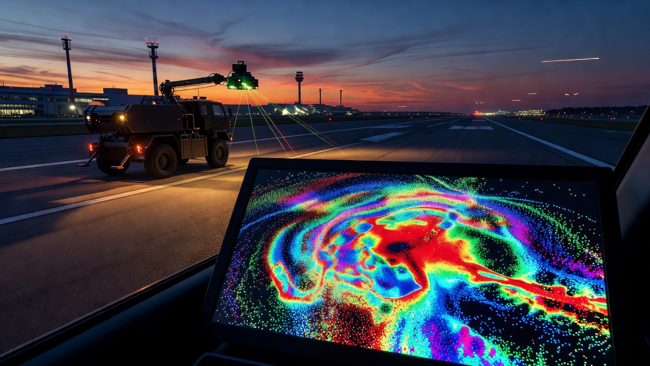
Time-of-flight (ToF) LiDAR, also called pulse-based or discrete-return LiDAR, emits short-duration laser pulses, typically nanoseconds in length, and measures the precise round-trip travel time of each pulse. The sensor’s timing electronics must resolve time intervals with picosecond accuracy to achieve millimeter-level ranging precision. A typical ToF LiDAR system emits between 50,000 and 2,000,000 pulses per second, with each pulse potentially generating multiple returns as the laser beam encounters partially transparent surfaces such as vegetation canopy, power lines, or glass. The first return corresponds to the first surface encountered, while the last return typically represents the ground or the most distant solid surface. Multi-return capability is a distinguishing advantage of ToF LiDAR for applications requiring terrain mapping beneath vegetation.
ToF scanners achieve the longest operational ranges of any LiDAR type, from 300 m for compact drone-mounted units to over 6,000 m for high-altitude airborne systems. The ranging accuracy depends on the pulse rise time, detector bandwidth, and signal-to-noise ratio, with typical single-shot precision ranging from 3 mm to 5 cm depending on the sensor class. The primary limitation of ToF LiDAR is the maximum measurement rate, which is constrained by the speed of light and the maximum unambiguous range, a sensor operating at 2 km range is limited to approximately 75,000 measurements per second because each pulse must complete its round trip before the next pulse can be emitted without ambiguity.
Phase-Shift (Continuous Wave) LiDAR
Phase-shift LiDAR, also called continuous wave (CW) or amplitude-modulated LiDAR, emits a constant laser beam whose intensity is modulated at one or more known frequencies. The sensor compares the phase of the transmitted modulation signal with the phase of the returned signal after reflection from the target. The phase difference is directly proportional to the distance, expressed by the formula: time of flight equals phase shift divided by (2π multiplied by modulation frequency). By using multiple modulation frequencies simultaneously, phase-shift systems resolve range ambiguities and extend their unambiguous measurement interval.
Phase-shift scanners acquire data at significantly higher rates than ToF systems, up to 1 million to 2 million measurements per second, because they do not wait for each pulse to return before emitting the next signal. This makes phase-shift technology ideal for applications requiring very dense point clouds in confined spaces, such as building interiors, bridge undersides, and tunnel linings. However, the effective range of phase-shift LiDAR is limited to approximately 80-150 m because the phase measurement becomes ambiguous at distances exceeding the modulation wavelength. Phase-shift systems also tend to exhibit higher noise levels in the point cloud compared with ToF sensors, manifesting as additional random scatter around true surface positions.
Pulse vs. Continuous Wave, Comparative Analysis
| Parameter | Time-of-Flight (Pulse) LiDAR | Phase-Shift (Continuous Wave) LiDAR |
|---|---|---|
| Measurement principle | Direct pulse timing | Phase comparison of modulated signal |
| Maximum range | 300 m to 6,000+ m | 80 m to 150 m |
| Measurement rate | 50,000 to 500,000 pts/s | 500,000 to 2,000,000 pts/s |
| Typical single-point precision | 3-10 mm at 100 m | 1-6 mm at 50 m |
| Multi-return capability | Yes (typically 3-5 returns) | No (single return) |
| Noise level | Lower | Higher |
| Primary applications | Airborne, mobile, long-range TLS | Architectural, industrial, short-range TLS |
| Sensitivity to ambient light | Moderate | Higher |
In practice, modern infrastructure inspection projects often combine both technologies, using phase-shift terrestrial scanners for detailed close-range structural documentation and pulse-based airborne or mobile scanners for broader corridor and topographic coverage.
Types of LiDAR Platforms for Infrastructure Inspection
The platform carrying the LiDAR sensor determines the coverage area, point density, accuracy, and operational constraints of the survey. Four primary platform categories serve infrastructure inspection applications, each with distinct characteristics.
Terrestrial Laser Scanning (TLS)
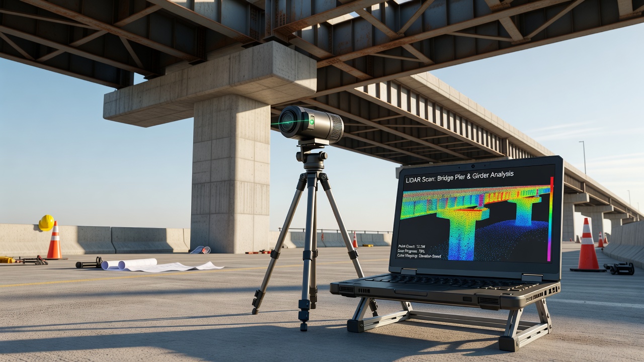
Terrestrial Laser Scanning (TLS) employs tripod-mounted laser scanners positioned at multiple survey stations around the target structure. Each scan collects a 360-degree horizontal by 270-320 degree vertical field of view, capturing all surfaces visible from the scanner position. Multiple scan positions are registered together using common targets or cloud-to-cloud registration algorithms to produce a complete 3D model of the infrastructure asset. TLS achieves the highest accuracy of any LiDAR platform, with typical single-point precision of 1-6 mm at ranges up to 100 m for phase-shift instruments and 3-10 mm at ranges up to 600 m for pulse-based long-range instruments.
For bridge inspection, TLS is positioned under the superstructure to capture bearing seats, girder bottom flanges, pier caps, and deck soffits, areas that are difficult to access with other platforms. For pavement evaluation, TLS is used for localized high-density reference sections to calibrate mobile LiDAR data or to document specific distress features at millimeter resolution. The primary limitations of TLS are the time required to set up and move between stations, the need for line-of-sight access to all surfaces, and the potential for incomplete coverage of overhead or shadowed areas.
Mobile LiDAR (MLS)
Mobile LiDAR Scanning (MLS) mounts laser scanners, GNSS receivers, and inertial measurement units (IMUs) onto vehicles such as survey vans, trucks, or rail carts. The system collects data while the vehicle moves at normal traffic speeds, typically 30-80 km/h for road surveys and 15-40 km/h for airport runway surveys. MLS systems typically incorporate two to eight laser scanner heads arranged to provide 360-degree horizontal coverage, capturing both the pavement surface and the surrounding corridor environment including signage, barriers, buildings, and vegetation.
The accuracy of MLS depends on the quality of the GNSS/IMU positioning solution. In open-sky conditions with good satellite visibility, absolute accuracy of 10-30 mm is achievable. In urban canyons, tunnels, or under dense tree canopy, accuracy degrades to 50-100 mm unless supplemental control measures are implemented. Modern MLS sensors capture 500,000 to 2 million points per second, generating point densities of 500-5,000 points per square meter on the pavement surface, sufficient for detailed roughness, rutting, and texture analysis.
MLS is the dominant platform for pavement condition assessment of highways, airport runways, and taxiways. The ability to survey entire airport pavement networks during a single overnight closure period, collecting full-width, full-length data at driving speeds, represents a transformative improvement over manual inspection methods that would require weeks of lane closures and walking inspections.
Airborne LiDAR (ALS)
Airborne LiDAR Scanning (ALS) mounts laser scanners on fixed-wing aircraft, helicopters, or gyrocopters. ALS systems combine the laser scanner with high-precision GNSS and IMU to determine the position and orientation of each laser pulse. The laser scans perpendicular to the flight direction using an oscillating mirror, rotating polygon, or fiber-optic array, creating a zigzag or parallel swath of measurements along the flight path. Typical flight altitudes range from 300 m to 3,000 m above ground level, producing swath widths of 300 m to 3,000 m depending on the scan angle and altitude.
ALS provides broad-area coverage unmatched by any other LiDAR platform. A single flight hour can cover 50-200 square kilometers depending on the point density requirements. For infrastructure inspection, ALS is used for corridor mapping of highways, railways, and power transmission lines, topographic base mapping for bridge and tunnel approaches, and obstacle surveys around airports for ICAO Annex 14 compliance. Typical ALS point densities range from 2 to 30 points per square meter, with vertical accuracy of 5-30 cm depending on flight parameters and ground control. The ASPRS Quality Level (QL) classification standardizes ALS data specifications: QL0 (5 cm RMSE, 8+ pts/m²), QL1 (10 cm RMSE, 8+ pts/m²), QL2 (10 cm RMSE, 2+ pts/m²), and QL3 (20 cm RMSE, 0.5+ pts/m²).
Drone-Mounted LiDAR (UAV LiDAR)
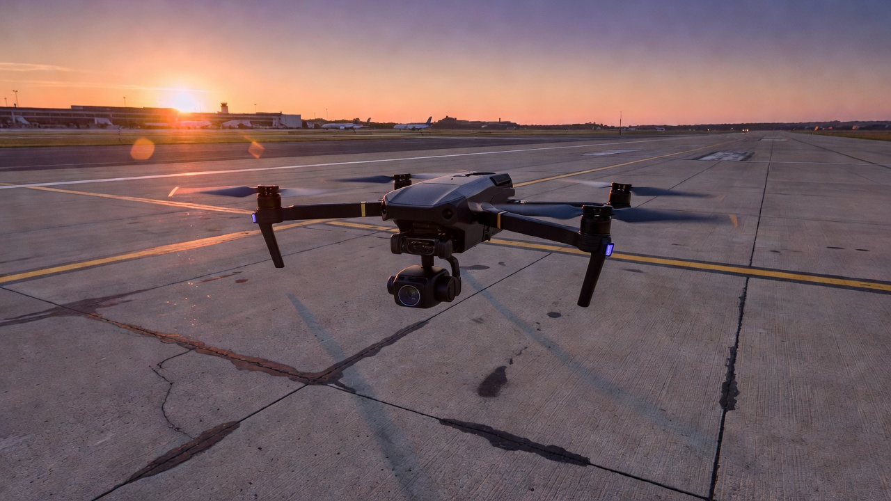
Drone-mounted LiDAR or UAV LiDAR bridges the gap between terrestrial and airborne platforms. Small, lightweight laser scanners, typically weighing 500 g to 2 kg, are integrated with survey-grade GNSS and IMU on unmanned aerial vehicles. UAV LiDAR operates at flight altitudes of 30-120 m above ground, covering 5-50 hectares per flight hour at point densities of 50-500 points per square meter.
UAV LiDAR is particularly valuable for infrastructure inspection in confined or elevated environments where terrestrial access is difficult and conventional aircraft cannot operate safely. Applications include bridge deck and superstructure inspection, quarry and stockpile volume calculation, building facade documentation, power line clearance measurement, and construction progress monitoring. The combination of high point density, flexible flight planning, and relatively low operational cost makes UAV LiDAR increasingly competitive with both TLS and MLS for many infrastructure inspection scenarios.
Point Cloud Density and Accuracy
Density Specifications
Point density, the number of LiDAR points per unit area (typically points per square meter), determines the level of geometric detail resolvable in the point cloud. Higher density enables detection of smaller surface features but increases data volume, processing time, and storage requirements. The required density for infrastructure inspection varies significantly by application:
| Application | Recommended Point Density | Minimum Feature Size Detectable |
|---|---|---|
| Regional topographic mapping | 0.5-2 pts/m² | 1-2 m |
| Airport obstacle limitation surfaces | 2-8 pts/m² | 30-50 cm |
| Pavement roughness (IRI) measurement | 50-200 pts/m² | 5-10 cm |
| Pavement rutting analysis | 200-500 pts/m² | 2-5 cm |
| Bridge clearance measurement | 500-1,000 pts/m² | 2-5 cm |
| Pavement texture (MPD) | 1,000-5,000 pts/m² | 1-3 mm |
| Concrete crack detection (TLS) | 10,000-100,000 pts/m² | 0.5-2 mm |
The relationship between point spacing and object detection follows the Nyquist sampling criterion: the point spacing should be at least half the size of the smallest feature to be reliably detected. If the point spacing is 10 mm, features smaller than approximately 20 mm may not be clearly resolved in the point cloud.
Accuracy Parameters
LiDAR accuracy is expressed through multiple metrics. Absolute accuracy describes how closely measured point coordinates match true ground positions relative to a defined coordinate reference system (e.g., WGS84, a national grid). It is assessed using Root Mean Square Error (RMSE) calculated against independently surveyed checkpoints, typically a minimum of 20-30 checkpoints distributed across the survey area. Relative accuracy describes the internal consistency of the point cloud, how well neighboring points align with each other without reference to external control.
For mobile and airborne LiDAR, two key relative accuracy metrics are monitored. Within-swath accuracy measures point-to-point consistency within a single flight line or vehicle pass. Swath-to-swath accuracy measures the alignment between overlapping adjacent passes, discrepancies here indicate systematic errors in the GNSS/IMU solution or calibration parameters.
The ASPRS Positional Accuracy Standards for Digital Geospatial Data define standard accuracy classes:
| Quality Level | Vertical Accuracy (RMSE at 95% Confidence) | Minimum Point Density |
|---|---|---|
| QL0 | 5 cm (RMSEz ≤ 2.5 cm) | 8 pts/m² |
| QL1 | 10 cm (RMSEz ≤ 5 cm) | 8 pts/m² |
| QL2 | 10 cm (RMSEz ≤ 5 cm) | 2 pts/m² |
| QL3 | 20 cm (RMSEz ≤ 10 cm) | 0.5 pts/m² |
| QL4 | 40 cm (RMSEz ≤ 20 cm) | 0.25 pts/m² |
| QL5 | 100 cm (RMSEz ≤ 50 cm) | 0.1 pts/m² |
Factors Affecting Accuracy
LiDAR accuracy is influenced by numerous factors across the data collection and processing chain. System calibration, the precise determination of boresight angles between the laser scanner, IMU, and GNSS antenna, is the most critical factor. Calibration errors as small as 0.01 degrees can produce horizontal displacement errors of 17 cm at 100 m range. Flight or driving parameters including altitude, speed, scan angle, and pulse repetition frequency all affect accuracy, lower altitude improves ranging precision and reduces the laser footprint on the ground. Terrain complexity affects ground classification accuracy, steep slopes, dense vegetation, and urban environments challenge automated ground filtering algorithms. Ground control quality, the number and distribution of surveyed checkpoints, directly determines the confidence in absolute accuracy assessment.
LiDAR Applications for Pavement Inspection
Pavement condition assessment is one of the most mature and economically significant applications of LiDAR in infrastructure inspection. Mobile LiDAR systems can survey entire runway, taxiway, and apron networks during a single operational window, generating comprehensive geometric data for multiple pavement condition metrics simultaneously.
International Roughness Index (IRI)
International Roughness Index (IRI) quantifies the longitudinal surface profile unevenness that affects ride quality and dynamic loading on aircraft landing gear or vehicle suspension. IRI is calculated from the accumulated suspension travel of a mathematical quarter-car model as it traverses a measured longitudinal profile at a standard speed of 80 km/h. LiDAR-derived IRI requires extracting a dense longitudinal elevation profile along the pavement surface, typically at 25 mm to 250 mm intervals depending on the desired precision. The LiDAR profile is filtered to remove wavelength components outside the IRI-sensitive band (0.5 m to 50 m), then processed through the quarter-car algorithm specified in ASTM E1926 and AASHTO M328.
For airport runways, ICAO Annex 14 specifies maximum allowable roughness values, and many national aviation authorities mandate regular IRI monitoring. Mobile LiDAR captures IRI for every lane or wheel track simultaneously across the full pavement width, producing color-coded roughness maps that identify localized undulations, settlement areas, and construction joint problems. Typical IRI values for new airport pavements range from 1.0 to 1.5 m/km, while values exceeding 2.5 m/km typically trigger rehabilitation planning. LiDAR-based IRI measurement correlates strongly with inertial profiler reference measurements, with typical differences of 0.1-0.2 m/km on well-calibrated systems.
Rutting Measurement
Rutting, permanent longitudinal depression in the wheel paths caused by repeated traffic loading, is a critical pavement distress that can accumulate water and create hydroplaning hazards on runways and high-speed roads. LiDAR measures rutting by extracting transverse cross-sectional profiles perpendicular to the pavement centerline at regular intervals (typically every 1-5 m). The rut depth is calculated as the maximum vertical deviation between the measured cross-section and a straight-edge or wire-line reference connecting the high points on either side of the rut.
Automated rutting analysis from mobile LiDAR point clouds processes thousands of transverse profiles per kilometer, generating continuous rut depth measurements along each wheel path. For airport runways, FAA and ICAO standards specify maximum allowable rut depths, typically 6-12 mm for critical surfaces depending on classification, with corrective action required when thresholds are exceeded. LiDAR-derived rutting measurements achieve repeatability of 1-2 mm, significantly outperforming manual straightedge measurements (typically 3-5 mm repeatability) and eliminating the subjectivity inherent in manual visual assessment.
Pavement Macrotexture
Pavement macrotexture, the surface texture with wavelength components from 0.5 mm to 50 mm, is critical for tire-pavement friction, particularly at high speeds and in wet conditions. LiDAR measures macrotexture using the Mean Profile Depth (MPD) methodology specified in ASTM E1845 and ISO 13473. A longitudinal or transverse profile is extracted from the point cloud, typically 100 mm in length. The profile is divided into two 50 mm segments, the average peak height is calculated for each segment, and the MPD is the average of these two values minus the profile’s mean elevation.
Mobile LiDAR systems with point densities exceeding 1,000 pts/m² on the pavement surface can compute MPD at full-lane-width coverage at driving speeds, correlating strongly with traditional laser profilometer measurements (typical R² > 0.85). For airport runways, ICAO Annex 14 specifies minimum surface texture depth requirements, typically 0.8-1.0 mm MPD for new surfaces. LiDAR-based macrotexture mapping identifies areas of accelerated polishing, inadequate grooving performance, or rubber contamination that require maintenance intervention such as grooving restoration, diamond grinding, or rubber removal.
Crack Detection and Quantification
LiDAR detects pavement cracks by identifying geometric discontinuities, abrupt changes in surface elevation or point cloud normal vectors that indicate the presence of open cracks. At typical mobile LiDAR point densities (100-500 pts/m²), cracks wider than 5-10 mm are detectable. Terrestrial LiDAR at close range with point densities exceeding 10,000 pts/m² can resolve cracks narrower than 1 mm.
From the point cloud, crack metrics including length, width, orientation, and density are extracted. Crack length is measured along the crack path in the pavement plane. Crack width at each point along the crack path is computed from the distance between the crack edges on either side. Crack orientation (longitudinal, transverse, diagonal, or random) is classified based on the angle relative to the pavement centerline. Crack density is the total crack length per unit area, used in Pavement Condition Index (PCI) calculations per ASTM D5340 and ASTM E3303 standards.
A significant advantage of LiDAR-based crack detection over camera-based methods is the ability to measure crack depth, the vertical opening of the crack below the surrounding pavement surface, which correlates with crack severity and structural significance. Camera-based systems can only detect crack presence and surface width, missing the critical third dimension of crack geometry.
LiDAR Applications for Bridge Inspection
Bridges represent one of the most demanding infrastructure inspection targets due to their geometric complexity, inaccessible areas, and critical safety implications. LiDAR provides comprehensive 3D documentation that supports multiple bridge inspection and monitoring objectives.
Vertical and Horizontal Clearance Measurement
Vertical clearance, the minimum distance between the bridge superstructure and the surface below (roadway, railway, or waterway), is a critical safety parameter for route planning and load permitting. LiDAR measures clearance by extracting the lowest point on the bridge superstructure (typically the bottom of the lowest girder or arch) and computing the vertical distance to the ground surface directly below. The full 3D nature of the point cloud enables identification of the minimum clearance envelope across the entire bridge width, accounting for cross-slope, superelevation, and structural camber.
Horizontal clearance, the clear distance between bridge abutments, piers, or barriers, is similarly extracted from the point cloud by measuring distances between vertical structural elements at critical elevations. For navigable waterways, horizontal clearance between piers and vertical clearance above high water are both required for vessel routing. LiDAR surveys conducted during navigation closures capture the as-built geometry with millimeter accuracy, replacing design-drawing assumptions with measured reality. Repeated clearance measurements over time reveal settlements, structural movements, or pavement overlay thickness changes that may reduce clearance below regulatory minimums.
Structural Deformation Monitoring (4D LiDAR)
4D LiDAR, repeated 3D scanning over time, is a powerful tool for detecting and quantifying structural deformation, settlement, rotation, and displacement. The principle is straightforward: the bridge is scanned at two or more time points using identical sensor positions and registration procedures, the resulting point clouds are aligned in a common coordinate system, and deviations between the scans are computed as deformation maps.
Deformation monitoring from TLS achieves sensitivity of 2-5 mm for bridges of typical span lengths (20-200 m) when proper error control procedures are followed. This enables detection of bearing settlement, pier rotation, girder deflection changes, and deck camber loss that may indicate structural distress. For long-span bridges, deformation monitoring over seasonal temperature cycles characterizes the normal thermal movement envelope, against which abnormal movements, indicating bearing failure, foundation settlement, or structural damage, can be detected.
Key metrics extracted from LiDAR deformation analysis include vertical deflection (change in elevation at midspan or quarter points), bearing displacement (horizontal and vertical movement at support locations), pier plumbness (verticality deviation), and deck profile change (loss of designed camber or sag development). Advanced analysis techniques including cross-sectional shape fitting, cylinder fitting for columns, and plane fitting for bearing surfaces provide sub-millimeter sensitivity for localized element deformation.
Element Geometry and Section Loss
LiDAR point clouds enable detailed geometric measurement of individual bridge elements including girders, bearings, piers, abutments, and deck components. Cross-sectional geometry of steel girders is extracted from the point cloud by slicing the bridge at regular intervals perpendicular to the girder axis. The flange widths, flange thicknesses, web depths, and web thicknesses are measured from the cross-sectional point cloud and compared with as-designed dimensions. Section loss due to corrosion, reduction in flange or web thickness, is detected as deviations between measured and expected dimensions, with sensitivity depending on point density and surface condition.
For reinforced concrete elements, LiDAR measures cover depth over reinforcement (where surface spalling exposes bars), crack widths and depths, and spalled area extent. The 3D nature of the point cloud enables volume calculation for spalled or delaminated concrete, directly informing repair quantity estimates. Bearing geometry, including sole plate dimensions, rocker or roller positions, and elastomeric pad thickness, is captured with sufficient detail to assess bearing condition and remaining movement capacity.
Deck Surface Condition
Bridge deck surface condition, including wear, cracking, rutting, and potholing, is assessed using the same pavement analysis techniques described for runways and roads. Mobile or terrestrial LiDAR captures the deck surface at sufficient density to compute IRI, rut depth, texture, and crack metrics. For bridge decks, an additional critical parameter is deck cross-slope, the transverse slope designed to drain water from the surface. LiDAR point clouds measure actual as-built cross-slope and identify areas of ponding or inadequate drainage that accelerate deck deterioration.
Deck joint condition is evaluated from the point cloud by measuring joint gap width, vertical alignment (step between adjacent spans), and seal condition. Expansion joint problems are a frequent contributor to deck deterioration, and LiDAR provides a quantitative, repeatable assessment method that replaces subjective visual inspection.
Point Cloud Processing for Infrastructure Inspection
Classification and Filtering
Raw LiDAR point clouds contain data from all surfaces within the sensor’s field of view, pavement, vegetation, vehicles, buildings, signage, and atmospheric noise. Point cloud classification assigns semantic labels to each point, enabling extraction of the specific surface or feature relevant to the inspection objective. The ASPRS LAS specification defines standard classification codes that ensure interoperability across software platforms: class 2 (ground), class 6 (building), class 8 (model key point for digital terrain model), class 9 (water), class 13 (wire, shield), class 14 (wire, conductor), and class 17 (bridge deck), among others.
Classification algorithms fall into three categories. Geometric rule-based methods use thresholds on attributes such as elevation, slope, intensity, return number, and local point density to separate ground from non-ground points. Progressive morphological filters and cloth-simulation filters are common geometric approaches. Machine learning classifiers including random forests, support vector machines, and gradient boosting operate on feature vectors computed for each point, eigenvalues of the local covariance matrix (linearity, planarity, sphericity), height above ground, intensity statistics, and multi-scale geometric descriptors. Deep learning methods, discussed in section 9, directly consume raw point coordinates and learn hierarchical spatial features.
Registration and Georeferencing
Registration is the process of aligning multiple individual scans into a single coherent point cloud. For TLS, registration uses either target-based methods (spheres, checkerboards, or tilt-and-turn targets placed in the overlap area between scans) or cloud-to-cloud methods (iterative closest point algorithm minimizing the distance between overlapping surfaces). Typical TLS registration accuracy is 1-5 mm for well-designed survey networks with adequate overlap (30-50% between adjacent scans).
Georeferencing ties the registered point cloud to a real-world coordinate system, typically a national grid or geographic coordinate reference system with elevation referenced to a vertical datum. For mobile and airborne LiDAR, georeferencing is inherent in the GNSS/IMU solution, but residual errors are corrected using surveyed ground control points. For TLS, georeferencing is achieved by scanning targets whose coordinates have been independently surveyed, or by matching the point cloud to reference data such as orthophotos or existing control networks. ICAO Annex 14 requires that aeronautical surveys including runway geometry and obstacle data be georeferenced to WGS84 coordinates.
Feature Extraction
Feature extraction transforms the classified point cloud into the specific measurements and metrics required for infrastructure inspection. Extraction algorithms operate on individual points, segments, or the entire classified surface:
- Elevation profiles are extracted along specified alignments (centerlines, wheel paths, gutter lines) by projecting points onto the alignment and interpolating elevation at regular intervals.
- Cross-sections are extracted perpendicular to the alignment at specified stations, typically using a swath width of 3-10 m and point spacing of 1-10 mm.
- Breaklines, linear features representing abrupt surface changes such as curbs, gutter edges, crack edges, and joint boundaries, are extracted by analyzing point cloud gradient and normal vector discontinuities.
- Planar surfaces (pavement patches, bridge deck segments, building walls) are identified using RANSAC or region-growing plane fitting algorithms, and their orientation (dip, dip direction, slope, aspect) is computed from the fitted plane parameters.
- Bare-earth models for terrain analysis are generated by classifying and removing non-ground points (vegetation, buildings, vehicles) using the classification procedures described above, then interpolating the remaining ground points into a continuous surface.
Data Formats and Management
LiDAR point clouds are stored in standardized formats that support efficient access, processing, and exchange. LAS/LAZ (LASzip compressed) is the primary format specified by ASPRS, supporting classification codes, intensity, return number, RGB color, and user-defined attributes. E57 is a vendor-neutral format supporting rich metadata including coordinate reference system, sensor calibration, and scan date. For large infrastructure inspections, the point cloud is often tiled into manageable geographic extents (e.g., 100 m x 100 m tiles) and organized in spatial index structures such as octrees or KD-trees for efficient query and visualization.
LiDAR vs. Photogrammetry for Infrastructure Inspection
Photogrammetry, the science of obtaining reliable measurements from photographs, is the primary alternative to LiDAR for 3D infrastructure documentation. Modern Structure-from-Motion (SfM) photogrammetry processes overlapping images captured from drones, aircraft, or ground-based cameras to reconstruct 3D geometry and produce orthorectified imagery. Understanding the comparative strengths and limitations of each technology is essential for selecting the appropriate method for specific inspection applications.
Comparative Analysis
| Parameter | LiDAR | Photogrammetry (SfM) |
|---|---|---|
| Measurement principle | Active laser pulse ranging | Passive image-based triangulation |
| Vertical accuracy | 1-30 mm (varies by platform) | 2-50 mm (varies with GCPs and camera) |
| Horizontal accuracy | 1-20 mm | 1-20 mm |
| Performance in low light | Fully operational | Severely degraded or non-functional |
| Performance in fog/haze | Moderate degradation | Severe degradation |
| Vegetation penetration | Yes (multi-return capability) | No (surface only) |
| Surface texture requirement | None (measures geometry directly) | Requires visible texture for matching |
| Color/RGB output | Optional (intensity only, or RGB if co-mounted camera) | Inherent (true orthoimagery) |
| Data collection speed | 50,000 to 2,000,000 pts/s | Limited by image capture rate |
| Processing time | Hours (direct measurements) | Days to weeks (image matching and bundle adjustment) |
| Hardware cost (drone system) | $50,000 - $350,000+ | $3,000 - $30,000 |
| Operating cost per km² | $200 - $2,000 | $50 - $500 |
Application-Specific Recommendations
For pavement roughness and rutting measurement, LiDAR is strongly preferred because the required geometric precision (1-3 mm vertical) is difficult to achieve reliably with photogrammetry, particularly on uniform pavement surfaces that lack the texture features needed for accurate image matching. Photogrammetric point clouds on low-texture asphalt or concrete typically exhibit higher noise levels (5-15 mm RMSE) that obscure the subtle elevation variations critical for IRI and rutting calculation.
For bridge clearance measurement, both technologies can achieve sufficient accuracy, but LiDAR offers faster data collection and direct geometric measurement without the computational expense of image matching. LiDAR also operates effectively in the shadowed areas beneath bridge superstructures where photogrammetry struggles due to low light and uniform surfaces.
For visual documentation and defect mapping, photogrammetry provides significant advantages. The colorized point clouds and orthophotos produced from photogrammetric surveys deliver visual context that aids inspector interpretation of defects. Camera-based crack detection on well-lit concrete surfaces can achieve higher resolution than typical mobile LiDAR, though specialized high-density TLS can compete at close range.
For vegetated corridors and terrain mapping, LiDAR’s multi-return capability provides unique value by penetrating vegetation to capture ground surface elevation, photogrammetry only captures the top of the vegetation canopy. For airport obstacle limitation surface surveys, LiDAR is the standard method for mapping terrain, trees, buildings, and other obstacles within the approach and departure surfaces.
Integrated Approaches
The most effective infrastructure inspection programs increasingly use integrated LiDAR-photogrammetry systems that mount both sensors on the same platform. The laser scanner provides precise geometry, while the camera provides high-resolution color texture. The combined dataset produces point clouds with accurate XYZ coordinates and realistic RGB color, supporting both quantitative analysis (roughness, clearance, deformation) and qualitative interpretation (defect identification, asset classification). Post-processing software such as Agisoft Metashape, Bentley ContextCapture, and DJI Terra supports simultaneous processing of LiDAR and photogrammetric data within unified workflows.
Integration with Visual Inspection
LiDAR data does not replace visual inspection but augments and enhances it. The point cloud provides the geometric framework and quantitative measurements, while visual inspection provides context, material assessment, and identification of defects that are not purely geometric, such as corrosion, delamination, spalling, and staining. Effective integration combines both data sources within a unified inspection workflow.
Point Cloud as Inspection Reference
The georeferenced point cloud serves as the spatial reference for all inspection observations. Inspectors navigate through the 3D point cloud in the office or field, marking observations, crack locations, spalled areas, corrosion patches, bearing problems, at their exact 3D positions. These observations are linked to the point cloud through geospatial coordinates or unique identifiers, creating a comprehensive digital inspection record that can be revisited, measured, and compared with future inspections.
Virtual Inspection Capability
High-density point clouds with integrated color photography enable virtual inspection, the ability to examine infrastructure assets remotely in 3D without physical site access. Virtual inspection is particularly valuable for bridges and structures in hazardous locations (over water, at height, in traffic), during periods of restricted access, or for preliminary assessment before mobilizing inspection crews. Studies have demonstrated that virtual inspection using combined LiDAR and photogrammetry data can identify 80-95% of significant defects compared with on-site inspection, depending on the defect type and point cloud quality.
The virtual inspection workflow involves loading the point cloud and associated imagery into specialized inspection software (such as ClearEdge3D Verity, Trimble RealWorks, or Leica Cyclone REGISTER), navigating to areas of interest using zoom, pan, and rotate controls, measuring defect dimensions directly from the point cloud, and documenting findings with annotations and screenshots. For routine inspections, the initial virtual assessment can identify areas requiring closer on-site investigation, optimizing the use of limited inspection resources.
AI-Based Point Cloud Analysis
Artificial intelligence, particularly deep learning, has transformed point cloud analysis over the past five years, enabling automated classification, segmentation, and defect detection at speeds and scales impossible with manual or rule-based methods.
Deep Learning Architectures for 3D Data
Deep learning networks designed for point cloud data must address the unique characteristics of 3D point sets: unordered point order, irregular density, and spatial sparsity. Three main architectural paradigms have emerged:
Point-based networks including PointNet and PointNet++ operate directly on raw point coordinates, learning per-point features through shared multilayer perceptrons and aggregating local features through hierarchical grouping. PointNet++ achieves state-of-the-art performance on semantic segmentation of infrastructure point clouds, with typical mean intersection-over-union (mIoU) scores of 65-75% for classes including ground, building, vegetation, bridge, and water.
Voxel-based networks convert the irregular point cloud into regular 3D voxel grids and apply 3D convolutional neural networks (CNNs). While voxelization introduces discretization artifacts, the regular grid structure enables efficient computation on GPU hardware. Sparse convolution techniques (e.g., MinkowskiEngine, TorchSparse) compute only on occupied voxels, dramatically reducing memory requirements compared with dense 3D convolutions.
Projection-based networks project the 3D point cloud into 2D representations, range images, bird’s-eye views, or spherical projections, and apply standard 2D CNNs. The projection approach leverages mature 2D computer vision architectures (ResNet, U-Net, EfficientNet) and large pretrained weights, but loses geometric information in the projection process.
Automated Pavement Distress Classification
AI models trained on labeled LiDAR point clouds automatically detect and classify pavement distress types. The models process point cloud tiles covering fixed pavement areas (typically 10 m x 10 m to 50 m x 50 m) and output distress type, severity, density, and location for each tile. Distress types classified include fatigue cracking (alligator pattern), block cracking, edge cracking, longitudinal and transverse cracking, rutting, depressions, corrugation, shoving, and polished aggregate.
The automated classification performance is evaluated using confusion matrices and precision-recall metrics. For common distress types with sufficient training data (1,000+ labeled examples), modern networks achieve precision of 80-95% and recall of 75-90%. Performance degrades for rare distress types and for distress features near the resolution limit of the point cloud. The classified distress data feeds directly into Pavement Condition Index (PCI) calculation per ASTM D5340 and ASTM E3303, replacing subjective manual visual assessment with objective, repeatable automated analysis.
Automated Bridge Element Recognition
For bridge inspection, deep learning models perform semantic segmentation of the point cloud into structural element classes: deck, girder, pier cap, column, abutment, bearing, barrier, and approach slab. Instance segmentation further distinguishes individual elements, identifying each girder as a separate instance for element-level condition assessment. Models trained on diverse bridge type datasets (steel girder, prestressed concrete, arch, cable-stayed, truss) achieve instance segmentation accuracy of 70-90% depending on bridge complexity and point cloud quality.
Automated element recognition enables several inspection automation capabilities. Element-specific condition assessment extracts geometric metrics (dimensions, alignment, deformation) for each recognized element and compares them with design values. Defect detection within elements identifies local geometric anomalies, section loss, corrosion pitting, cracking, spalling, within each element. Change detection between inspections compares element geometry and defect presence between consecutive inspection cycles, quantifying deterioration rates and informing maintenance prioritization.
Change Detection and Temporal Analysis
AI-based change detection algorithms compare point clouds from successive inspection campaigns to identify new or progressing defects. Rigid registration of multi-temporal point clouds using ICP on stable reference features aligns the datasets, after which the algorithm computes the signed distance between each point in the new survey and the corresponding surface in the baseline survey. Changes exceeding a detection threshold (typically 3-10 mm depending on noise level) are flagged for inspection review.
For pavement monitoring, change detection identifies new crack development, crack width increase, rut progression, and surface wear. For bridge monitoring, it identifies bearing displacement, girder deflection change, pier settlement, and deck profile deterioration. Temporal analysis over multiple inspection cycles (3-5 years of data) enables deterioration rate modeling and remaining service life prediction, supporting data-driven maintenance planning and capital investment prioritization.
Summary
LiDAR has become an indispensable technology for infrastructure inspection, providing accurate, dense, and repeatable 3D geometric data that complements and enhances traditional visual inspection methods. From pavement roughness measurement at highway speeds to millimeter-scale bridge deformation monitoring, LiDAR delivers quantitative condition data that supports objective, data-driven infrastructure management decisions. The integration of LiDAR with photogrammetry, visual inspection, and AI-based automated analysis creates comprehensive inspection workflows that improve safety, reduce cost, and extend asset service life. As sensor technology continues to advance, with smaller, lighter, faster, and more accurate LiDAR systems entering the market, the role of laser scanning in infrastructure inspection will continue to expand, driving the transition from subjective manual inspection to objective digital condition assessment.
For expert guidance on implementing LiDAR-based inspection solutions for your pavement, bridge, runway, or other infrastructure assets, contact our team or schedule a demo .
Frequently Asked Questions
- What is the difference between time-of-flight and phase-shift LiDAR?
- Time-of-flight (pulse-based) LiDAR emits short laser pulses and measures the travel time to calculate distance. It operates effectively over long ranges (up to several kilometers) and is used in airborne, mobile, and long-range terrestrial applications. Phase-shift LiDAR emits a continuous modulated laser wave and measures the phase shift between transmitted and received signals to determine distance. Phase-shift scanners acquire data much faster, up to 1 million points per second, but their effective range is limited to approximately 100 meters. Phase-shift systems also tend to produce more noise in the point cloud compared to time-of-flight systems.
- How accurate is LiDAR for infrastructure inspection?
- LiDAR accuracy depends on the platform, sensor calibration, and ground control. Terrestrial laser scanners (TLS) achieve the highest accuracy with typical single-point precision of 1-6 mm at 100 m range. Mobile LiDAR systems mounted on vehicles achieve 5-20 mm relative accuracy and 10-50 mm absolute accuracy. Airborne LiDAR typically delivers 5-30 cm vertical accuracy depending on flight altitude and ground control density. The ASPRS (American Society for Photogrammetry and Remote Sensing) defines standardized quality levels: QL0 (5 cm RMSE), QL1 (10 cm RMSE), QL2 (10 cm RMSE), and QL3 (20 cm RMSE), each with associated point density requirements.
- What is the difference between LiDAR and photogrammetry for infrastructure inspection?
- LiDAR uses active laser pulses to directly measure 3D geometry, making it effective in low-light conditions, fog, and through vegetation canopy. It delivers superior vertical accuracy (1-3 cm vs 2-4 cm for photogrammetry) and does not require surface texture for feature matching. Photogrammetry reconstructs 3D geometry from overlapping photographs using structure-from-motion algorithms. It produces visually rich colorized point clouds at lower hardware cost (under $5,000 vs over $50,000 for LiDAR), but struggles in low-light, uniform surfaces, and vegetated areas. For infrastructure inspection, LiDAR is preferred for high-precision geometric measurements such as bridge clearance and pavement rutting, while photogrammetry excels in visual documentation and orthomosaic generation.
- How is LiDAR used for pavement condition assessment?
- LiDAR measures pavement surfaces by capturing millions of elevation points per second. From these point clouds, engineers extract International Roughness Index (IRI) by analyzing longitudinal elevation profiles, rutting depth by measuring transverse cross-slope deviations, macrotexture depth using Mean Profile Depth (MPD) calculations, and crack geometry by identifying discontinuities in the surface. Mobile LiDAR systems can survey entire runways or highways at highway speeds, generating data that feeds directly into Pavement Condition Index (PCI) calculations per ASTM E3303 standards. The technology replaces subjective manual inspection with objective, repeatable numerical measurements.
- How is LiDAR used for bridge inspection?
- LiDAR enables comprehensive geometric documentation of bridges including clearance measurement under the superstructure, vertical and horizontal alignment verification, deck surface profiling, bearing and girder geometry, and detection of structural deformations. Repeated scans over time (4D monitoring) reveal millimeter-scale movements, settlements, and rotations that indicate structural distress. Terrestrial laser scanning from fixed positions captures underside details, while mobile or drone-mounted LiDAR efficiently documents deck surfaces and fascia. LiDAR-based bridge inspection is a core component of Structural Health Monitoring (SHM) programs worldwide.
- What is point cloud classification in LiDAR processing?
- Point cloud classification is the process of assigning semantic labels to individual points in a LiDAR dataset, such as ground, vegetation, building, bridge, water, or noise. Classification enables extraction of specific features for analysis, such as isolating ground points for digital terrain models or bridge points for structural measurements. Traditional classification uses geometric rules and manual editing, while modern approaches employ machine learning and deep neural networks (e.g., PointNet++, RandLA-Net, KPConv) that learn to recognize spatial patterns directly from the 3D data. The ASPRS LAS specification defines standard classification codes (e.g., class 2 = ground, class 6 = building) ensuring interoperability across software platforms.
- Can LiDAR detect cracks in infrastructure?
- LiDAR point clouds can detect cracks and surface discontinuities, but the capability depends on point density and accuracy. Terrestrial LiDAR with point spacing under 1 mm at close range can identify cracks wider than 1-2 mm, especially when combined with intensity data that highlights material changes. Mobile LiDAR typically captures point spacing of 5-20 mm, sufficient for identifying structural cracks wider than 5-10 mm but not fine hairline cracking. For micro-crack detection, LiDAR is often complemented with high-resolution photography, infrared thermography, or ultrasonic testing. Advanced algorithms analyze point cloud normals and curvature to automatically detect crack-like discontinuities in bridge and pavement surfaces.
- What are the different types of LiDAR platforms?
- The four main LiDAR platform types are: (1) Terrestrial Laser Scanning (TLS), tripod-mounted stationary scanners providing the highest accuracy for localized bridge or building surveys, (2) Mobile LiDAR (MLS), vehicle-mounted systems scanning roads, runways, and tunnels at speed with 360-degree coverage, (3) Airborne LiDAR (ALS), aircraft or helicopter-mounted systems covering large areas for topographic and corridor mapping, and (4) Drone/UAV LiDAR, unmanned aerial vehicle-mounted lightweight scanners bridging the gap between terrestrial and airborne, ideal for confined or elevated structures.
- How does LiDAR integrate with AI for automated inspection?
- Modern LiDAR inspection workflows leverage deep learning for automated point cloud analysis. Neural network architectures like PointNet++, RandLA-Net, and KPConv perform semantic segmentation (assigning each point a class label) and instance segmentation (distinguishing individual objects). For pavement inspection, AI models automatically detect and classify crack types (longitudinal, transverse, alligator), measure rutting severity, and compute IRI. For bridges, AI identifies structural elements (girders, bearings, piers, deck) and detects anomalies such as spalling, corrosion, or deformation. These automated pipelines reduce processing time from weeks to hours and eliminate subjective variability in manual interpretation.
- What standards govern LiDAR data accuracy and quality?
- The primary standards governing LiDAR data include: ASPRS Positional Accuracy Standards for Digital Geospatial Data, defining Quality Levels QL0 through QL5 with specific RMSE and point density thresholds, ICAO Annex 14, specifying aeronautical survey requirements for airport pavements, obstacle limitation surfaces, and runway geometry, ASTM E3303, standard practice for calculating Pavement Condition Index using automated methods including LiDAR, and ISO 19157, geographic information data quality standards covering completeness, logical consistency, positional accuracy, temporal accuracy, and thematic accuracy.
- What is the typical point density required for infrastructure inspection?
- Required point density varies by application. For general topographic mapping: 2-8 points/m² (QL2-QL3). For pavement roughness and rutting analysis: 50-500 points/m² from mobile LiDAR. For bridge clearance and deformation: 1,000-10,000 points/m² from terrestrial scanning. For crack detection in concrete: 10,000-100,000 points/m² from close-range TLS. Higher point density improves small-feature resolution but increases data volume and processing time. Modern LiDAR sensors capture 500,000 to 2 million points per second, making dense surveys practical even for large infrastructure assets.
- Can LiDAR data be used to create digital twins of infrastructure?
- Yes. LiDAR point clouds form the foundational geospatial layer for infrastructure digital twins. The point cloud provides accurate as-built geometry that is used to create 3D BIM (Building Information Modeling) models, surface meshes, and CAD drawings. Digital twins combine LiDAR geometry with asset management databases, sensor data (strain gauges, temperature, vibration), and inspection records to provide a comprehensive, live digital representation of physical infrastructure. For airports, LiDAR-derived digital twin runways enable real-time pavement condition monitoring, maintenance planning, and compliance verification against ICAO Annex 14 standards.
This is a reference entry. TarmacView provides drone inspection services and doesn't sell the equipment or materials described in this glossary.