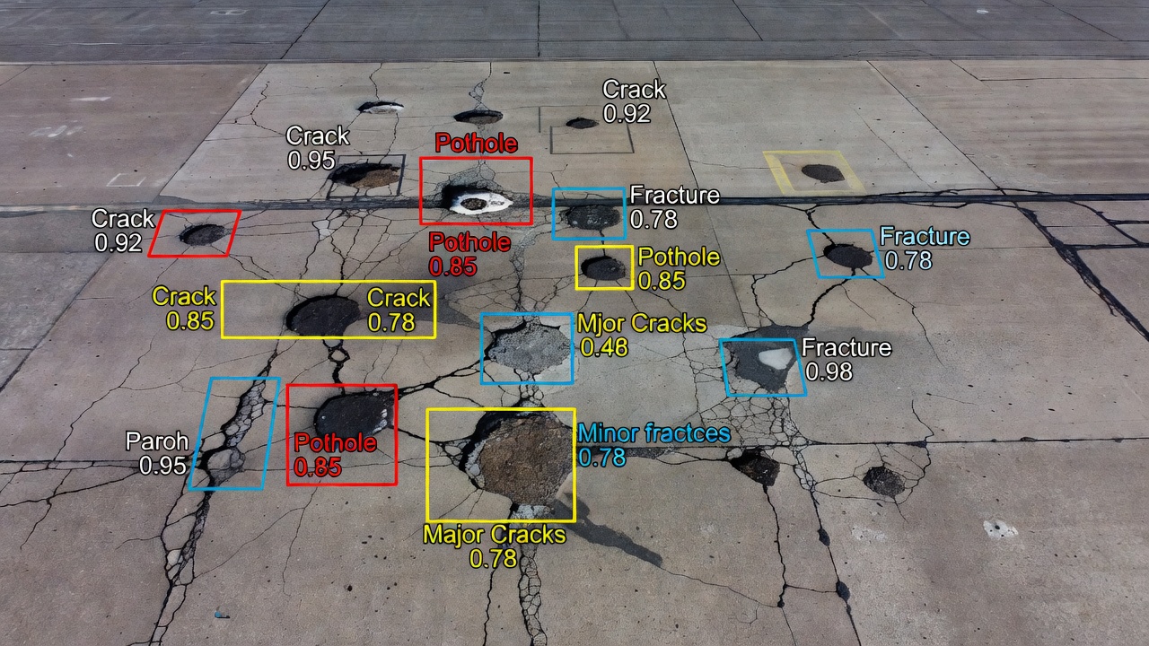
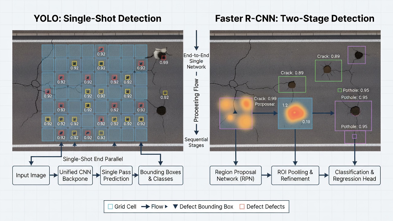
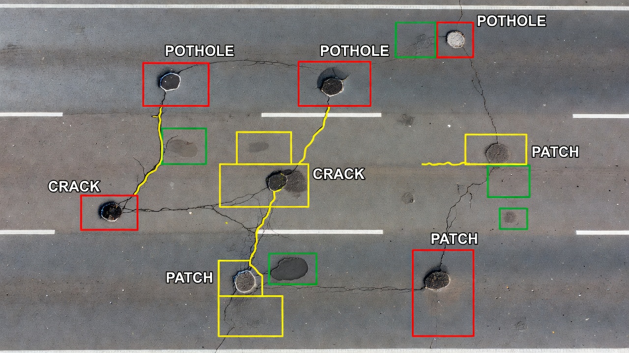
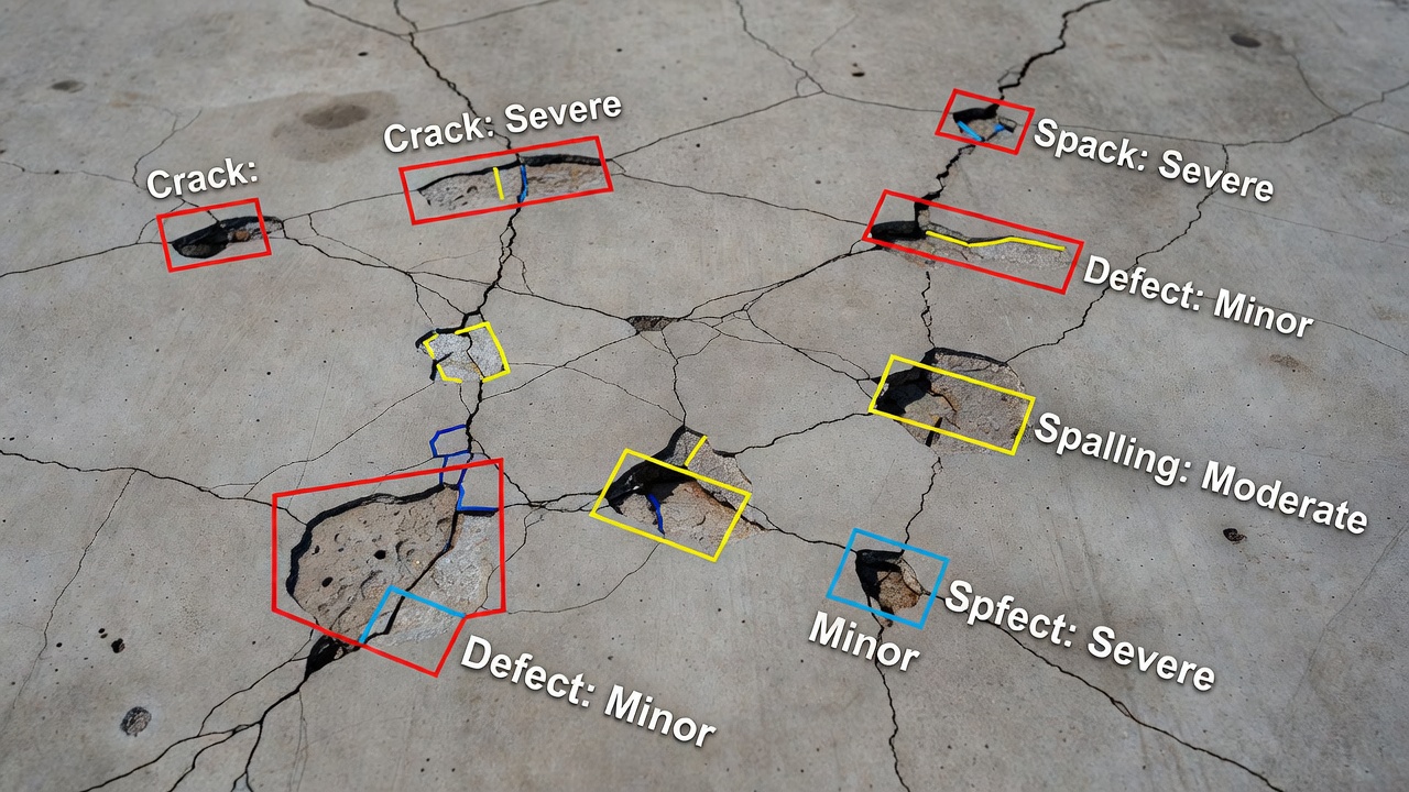
Semantic Segmentation for Infrastructure Scene Understanding
Semantic segmentation assigns a category label to every pixel in an image, enabling full-scene understanding for infrastructure inspection. Covers encoder-decod...
Object detection locates and classifies objects in images using bounding boxes — for infrastructure inspection, this includes potholes, patches, signs, FOD, and large defects. YOLO, Faster R-CNN, and DETR are leading architectures. Covers object detection methods, training with bounding box annotations (VOC, COCO formats), evaluation metrics (mAP), and deployment for real-time inspection.
{
Object detection is a computer vision task that identifies and localizes objects within an image or video frame by drawing axis-aligned rectangles — called bounding boxes — around each detected item and assigning a class label with a confidence score. Unlike image classification which produces a single label for the entire image, object detection produces a variable-length list of detections, one per object instance present in the scene. For infrastructure inspection, these detected objects can include potholes, spalls, patches, construction joints, pavement markings, runway signage, and foreign object debris (FOD).
The output of an object detection model for a single input image is structured as a list of N detections, where each detection contains three components. The first component is the bounding box, typically represented as either (x_min, y_min, x_max, y_max) in pixel coordinates where (0,0) is the top-left corner, or as (x_center, y_center, width, height) in normalized coordinates where all values range from 0 to 1 relative to image dimensions. The second component is the class label, which is the index or name of the object category assigned to the detection — for example, class_id=0 for “pothole”, class_id=1 for “crack”, class_id=2 for “FOD”, and so on. The third component is the confidence score, a floating-point value between 0.0 and 1.0 representing the model’s estimated probability that an object of the predicted class is present within the bounding box at the correct location. Confidence scores at or above a defined detection threshold (typically 0.25 to 0.5 depending on the application) are accepted as valid detections, while scores below the threshold are discarded.
Mathematically, an object detection model implements a mapping function: f: I → {(b₁, c₁, s₁), (b₂, c₂, s₂), …, (b_N, c_N, s_N)}, where I is the input image, b_i is the bounding box vector, c_i is the class index, and s_i is the confidence score for detection i. The number of detections N varies per image depending on the number of objects present and the model’s detection sensitivity.
The bounding box is defined by four coordinates. In the COCO convention (used by Microsoft COCO dataset and most modern frameworks), the bounding box is [x, y, width, height] where (x, y) is the top-left corner of the box in absolute pixel coordinates. In the Pascal VOC convention, the bounding box is [x_min, y_min, x_max, y_max] — the coordinates of the top-left and bottom-right corners. In YOLO format, the bounding box is [x_center, y_center, width, height] in normalized coordinates (divided by image width and height), making the representation resolution-independent. The conversion between these formats is explicit. From COCO or VOC format, the bounding box area is computed as area = width × height, and the intersection over union (IoU) between two boxes is defined as the area of their overlap divided by the area of their union — the fundamental matching metric for evaluating detection quality.
For infrastructure inspection applications governed by ICAO Annex 14, Volume I (Aerodrome Design and Operations) and ASTM D5340 (Standard Test Method for Airport Pavement Condition Index Surveys), object detection must achieve localization accuracy suitable for defect counting and severity classification. A detection of a pothole on a runway surface, for example, must have a bounding box that tightly encloses the defect opening. If the bounding box significantly overestimates the defect area (including too much intact pavement), or underestimates it (cutting off part of the defect), the subsequent severity classification derived from spatial measurements will be inaccurate. The tightness of bounding box fit around infrastructure defects is measured by IoU against a manually annotated ground truth box — values above 0.7 are considered good for most infrastructure applications.

Object detection architectures are broadly categorized into three families: single-shot detectors, two-stage detectors, and transformer-based detectors. Each family makes distinct trade-offs between detection accuracy, inference speed, computational cost, and ease of training.
YOLO (You Only Look Once), introduced by Joseph Redmon et al. at the University of Washington in 2016, revolutionized object detection by reframing it as a single regression problem —直接从 image pixels to bounding box coordinates and class probabilities in a single forward pass of a neural network. Instead of running a classifier across multiple image regions as previous methods did, YOLO divides the input image into an S×S grid (typically 7×7 in the original version, but finer grids in later iterations). Each grid cell is responsible for predicting B bounding boxes (typically 2-3 in early versions) and C class probabilities, along with a confidence score for each box indicating how confident the model is that the box contains an object and how accurate the predicted box is.
The original YOLO architecture uses a convolutional neural network with 24 convolutional layers followed by 2 fully connected layers, inspired by the GoogLeNet architecture but with fewer parameters. The network processes the entire image in a single shot, giving YOLO its name and its primary advantage: speed. YOLO achieved 45 FPS on a Titan X GPU with 63.4 mAP on Pascal VOC 2007 — far faster than any contemporary detector.
YOLO evolution has been dramatic. YOLOv2 (YOLO9000, 2017) introduced anchor boxes with k-means clustering of dataset bounding boxes for better priors, batch normalization, and multi-scale training. YOLOv3 (2018) replaced the backbone with Darknet-53 incorporating residual connections and feature pyramid networks (FPN) for detecting objects at multiple scales, achieving 57.9 mAP@0.5 on COCO. YOLOv4 (2020) introduced the CSPDarknet53 backbone, Mish activation, and the Bag-of-Freebies (BoF) and Bag-of-Specials (BoS) training techniques including Mosaic data augmentation, DropBlock regularization, and CIoU loss. YOLOv5, developed by Ultralytics, introduced a PyTorch-based implementation with an easy-to-use training framework that became the industry standard for applied object detection.
YOLOv8 (2023) brought anchor-free detection, decoupled classification and regression heads, and a task-aligned assigner for positive/negative sample matching. YOLOv8x achieves 53.9 mAP on COCO at 280 FPS on a T4 GPU. YOLO11 (September 2024) introduced further optimization with improved backbone and neck design, achieving 54.7 mAP with 26.4 million parameters at 314 FPS. YOLO26 (September 2025) is the latest evolution, achieving approximately 56-57 mAP on COCO with inference speeds exceeding 350 FPS on modern GPUs. Each generation has improved the speed-accuracy Pareto frontier, making YOLO the dominant architecture for real-time infrastructure inspection.
The Ultralytics YOLO training framework (yolo CLI, ultralytics Python package) supports detection, segmentation, classification, pose estimation, and oriented bounding box (OBB) tasks under a unified API. For infrastructure inspection, YOLO detection models are trained using the command yolo train data=dataset.yaml model=yolo11x.pt epochs=200 imgsz=640. The framework automatically handles data loading, augmentation (Mosaic, MixUp, HSV jitter, rotation, scaling), learning rate scheduling (cosine decay), and metric logging. Export to ONNX, TensorRT, CoreML, and OpenVINO formats for edge deployment is built-in.
Faster R-CNN, introduced by Shaoqing Ren, Kaiming He, Ross Girshick, and Jian Sun at Microsoft Research (NIPS 2015), is the foundational two-stage object detector that established the dominant paradigm for high-accuracy detection before the rise of single-shot and transformer-based methods. It remains widely used for infrastructure inspection applications where accuracy is prioritized over speed.
The Faster R-CNN architecture operates in two stages. In the first stage, a Region Proposal Network (RPN) scans the feature maps produced by a backbone CNN (typically ResNet-50, ResNet-101, or ResNeXt) and proposes candidate object regions called Regions of Interest (RoIs). The RPN is itself a fully convolutional network that slides a small network window over the convolutional feature map, predicting k anchor boxes at each spatial location — typically k=9 anchor boxes of three scales (128², 256², 512²) and three aspect ratios (1:1, 1:2, 2:1). For each anchor, the RPN outputs an objectness score (probability that the anchor contains an object vs. background) and bounding box regression offsets (4 values refining the anchor box to better fit the object). The RPN is trained end-to-end with the detection network, sharing convolutional features, which is Faster R-CNN’s key innovation over the previous Fast R-CNN which used external selective search for region proposals.
In the second stage, each RoI from the RPN is processed through an RoIPool layer that extracts a fixed-size feature map (typically 7×7) from each region. These fixed-size feature maps are fed into fully connected layers — a classification head that predicts class probabilities (K object classes + background) and a bounding box regression head that outputs refined bounding box coordinates for each class. The loss function combines four components: RPN classification loss (binary cross-entropy for objectness), RPN regression loss (smooth L1 for box offsets), detection classification loss (cross-entropy for class), and detection regression loss (smooth L1 for refined boxes).
Faster R-CNN with a ResNet-101-FPN backbone achieves 59.1 AP on COCO test-dev (per Mask R-CNN benchmark). Inference speed ranges from 5-15 FPS depending on backbone depth and input resolution. For infrastructure defect detection, Faster R-CNN has been demonstrated to achieve higher accuracy than YOLO for small defects (<32² pixels in the input image) due to its two-stage design that focuses the second-stage classifier specifically on proposed regions rather than the entire image grid.
The primary disadvantage of Faster R-CNN for infrastructure inspection is inference speed. At 5-15 FPS, it cannot process full-rate video streams (30 FPS) without frame-skipping, making it unsuitable for real-time inspection from fast-moving vehicles or UAVs. However, for offline analysis of captured inspection imagery where processing time is not constrained, Faster R-CNN remains a strong choice for maximum per-image accuracy.
SSD (Single Shot MultiBox Detector), introduced by Wei Liu et al. at ECCV 2016, was the first high-performance single-shot detector that rivaled two-stage detector accuracy while maintaining real-time speed. SSD operates by predicting bounding boxes and class probabilities directly from feature maps at multiple scales without the region proposal stage.
The SSD architecture uses a base network (typically VGG-16 truncated at conv5_3, or MobileNet) followed by a series of additional convolutional layers that progressively reduce spatial resolution. Detections are made from feature maps at 6 different scales — conv4_3 (38×38), conv7 (fc7, 19×19), conv8_2 (10×10), conv9_2 (5×5), conv10_2 (3×3), and conv11_2 (1×1). At each feature map location, SSD predicts offsets for k default boxes (similar to anchor boxes) and per-class confidence scores. With 8732 default boxes across all feature maps, SSD provides dense coverage of the image at multiple scales.
The multi-scale design is SSD’s key contribution: larger feature maps (38×38) detect small objects while smaller feature maps (1×1) detect large objects. This hierarchical detection mechanism is conceptually similar to Feature Pyramid Networks (FPN) that would become standard in later detectors.
SSD300 (300×300 input) achieves 77.2 mAP on Pascal VOC 2007 at 46 FPS on a Titan X, while SSD512 (512×512 input) achieves 79.8 mAP at 19 FPS. On COCO, SSD512 achieves 31.2 AP. For infrastructure inspection, SSD has been applied to vehicle-mounted road defect detection with reported performance of 48-52 mAP@0.5 on pothole detection datasets.
DETR (Detection Transformer), introduced by Nicolas Carion, Francisco Massa, and the Facebook AI Research team at ECCV 2020, fundamentally rethinks object detection by eliminating many hand-crafted components that dominated previous architectures — anchor boxes, region proposals, non-maximum suppression (NMS), and IoU-based matching. DETR instead treats object detection as a direct set prediction problem using a transformer encoder-decoder architecture.
The DETR architecture has three components. A backbone CNN (typically ResNet-50 or ResNet-101) extracts a feature map from the input image. A transformer encoder processes the feature map through multi-head self-attention layers, allowing each position in the feature map to attend to all other positions — building a global understanding of the image context. A transformer decoder takes a set of N learned object queries (typically N=100 fixed vectors) and processes them through self-attention (queries attending to other queries) and cross-attention (queries attending to the encoder output). Each query learns to predict a specific object instance. The decoder outputs N predictions, each consisting of a class label (K classes + ∅ for no-object) and a bounding box. During training, a Hungarian loss matches the N predictions to the ground truth objects using bipartite matching — finding the optimal one-to-one assignment between predictions and true objects that minimizes total loss.
DETR’s core innovation is that the set prediction framework eliminates the need for duplicate suppression. Because the Hungarian matching enforces one-to-one assignment during training, the model naturally learns to output unique detections without requiring NMS post-processing. This simplifies the detection pipeline and removes a hyperparameter (NMS IoU threshold) that needs tuning per application.
DETR with ResNet-50 backbone achieves 42.0 AP on COCO with 50 FPS on an NVIDIA V100 GPU with a batch size of 1. Deformable DETR (Zhu et al., ICLR 2021) improved training convergence (10× faster) and small-object detection by replacing standard attention with deformable attention that attends only to a sparse set of key sampling points near each query. DINO (Zhang et al., CVPR 2023) further improved DETR to achieve 63.2 AP on COCO — the first detector to exceed 63 AP — using a contrastive denoising training approach and improved query initialization. RF-DETR (Roboflow, March 2025) became the first real-time detector to exceed 60 AP (60.5 AP@0.50 :0.95 at 25 FPS on T4), specifically optimized for practical deployment.
For infrastructure inspection, DETR-family detectors are promising because the transformer’s global attention mechanism can capture long-range spatial relationships — a crack at one end of the image may be part of the same defect network as another crack at the opposite end, and the transformer’s self-attention can model this dependency. However, practical adoption has been slower than YOLO due to higher GPU memory requirements and the need for specialized training infrastructure.
| Architecture | Type | COCO mAP@0.50 :0.95 | Speed (FPS) | Strengths for Infrastructure |
|---|---|---|---|---|
| YOLOv8x | Single-shot CNN | 53.9 | 280 | Real-time inspection, edge deployment, easy training |
| YOLO11x | Single-shot CNN | 54.7 | 314 | Best speed-accuracy, native Ultralytics ecosystem |
| YOLO26x | Single-shot CNN | ~57 | 350+ | Latest generation, improved small object detection |
| Faster R-CNN R101-FPN | Two-stage CNN | 59.1 | 8-12 | Highest per-image accuracy, offline analysis |
| SSD512 | Single-shot CNN | 31.2 | 19 | Lightweight, low memory requirements |
| Deformable DETR | Transformer | 46.2 | 10-15 | No NMS, global context awareness |
| DINO | Transformer | 63.2 | 8-10 | State-of-the-art accuracy, research benchmark |
| RF-DETR | Transformer | 60.5 | 25 | Real-time transformer detection, practical deployment |
Training object detection models requires ground truth annotations — manually labeled bounding boxes and class labels for every object instance in the training images. The format in which these annotations are stored affects dataset interoperability, conversion overhead, and tool compatibility.
The Pascal VOC (Visual Object Classes) format, developed for the annual VOC challenge (2005-2012), uses an XML file per image. Each XML file contains the image metadata (filename, size) and a list of object annotations with bounding boxes. The schema is:
<annotation>
<folder>images</folder>
<filename>pothole_001.jpg</filename>
<source><database>RunwayDefects</database></source>
<size><width>1920</width><height>1080</height><depth>3</depth></size>
<object>
<name>pothole</name>
<pose>Unspecified</pose>
<truncated>0</truncated>
<difficult>0</difficult>
<bndbox>
<xmin>342</xmin><ymin>156</ymin>
<xmax>521</xmax><ymax>378</ymax>
</bndbox>
</object>
<object>
<name>crack</name>
<bndbox>
<xmin>890</xmin><ymin>234</ymin>
<xmax>1245</xmax><ymax>256</ymax>
</bndbox>
</object>
</annotation>
Each <object> element contains: name — the class label string; pose — approximate pose descriptor (Frontal, Rear, Left, Right, Unspecified); truncated — binary flag indicating whether the object is cut off by the image boundary (0=no, 1=yes); difficult — binary flag for objects considered difficult to recognize even for humans (often excluded during evaluation); and bndbox — the bounding box in (xmin, ymin, xmax, ymax) pixel coordinates.
The VOC format has the advantage of human-readability and per-file independence (annotations can be created, copied, and modified as separate files without parsing a monolithic database). The disadvantage is that large datasets with thousands of images require storing thousands of XML annotation files, which can slow down loading and processing in data pipelines.
VOC format is predominantly used with Faster R-CNN and SSD implementations in Detectron2 (Meta), mmdetection, and older TensorFlow Object Detection API pipelines. Conversion from VOC to COCO JSON format is supported by all major data management tools including Roboflow, CVAT, and labelImg.
The COCO (Common Objects in Context) JSON format, introduced by Microsoft with the MS COCO dataset (2015), is the most widely used annotation format for modern object detection models. All annotations for the entire dataset are stored in a single JSON file with a hierarchical structure containing four top-level arrays.
The info dictionary contains metadata about the dataset — year, version, description, contributor, URL, and date_created. The licenses array lists image license information with id, name, and URL for each license type. The categories array defines the class taxonomy, where each entry has an id (integer, typically starting from 1), name (class label string), and supercategory (higher-level grouping, e.g., “defect” for “pothole”, “crack”, “spall”). The images array lists every image in the dataset with id (unique integer), file_name (relative path), height and width (in pixels), and optionally date_captured and license. The annotations array is the core data structure, where each entry contains: id (unique annotation identifier), image_id (reference to the parent image), category_id (reference to the category), bbox (bounding box as [x, y, width, height] in pixel coordinates — where (x, y) is the top-left corner), area (computed as width × height in pixels), segmentation (polygon or RLE format; empty array [] for detection-only datasets), and iscrowd (flag: 0 for individual objects, 1 for groups of uncountable objects).
The COCO JSON format’s single-file structure makes dataset loading fast (one file read vs. thousands), enables efficient random access by using image_id as an index, and is the standard input format for Detectron2, MMDetection, and the torchvision reference detection pipeline. All major annotation tools (CVAT, Labelbox, Supervisely, Roboflow, Scale AI) support COCO JSON export.
The COCO evaluation server uses this same JSON structure for submitting detection results, ensuring consistency between training data and evaluation data.
The YOLO format, developed by the Ultralytics team for their YOLO training framework, uses one plain-text TXT file per image. Each line in the file corresponds to one object detection and follows the format:
<class_id> <x_center> <y_center> <width> <height>
All values are floating-point numbers normalized to the range [0, 1] by dividing by the image width (for x_center and width) and height (for y_center and height). For example, a pothole with absolute bounding box (x_min=342, y_min=156, x_max=521, y_max=378) in a 1920×1080 image converts to: x_center = (342+521)/2/1920 = 0.2247, y_center = (156+378)/2/1080 = 0.2472, width = (521-342)/1920 = 0.0932, height = (378-156)/1080 = 0.2056 — resulting in annotation line: “0 0.2247 0.2472 0.0932 0.2056”.
The YOLO format’s advantages are extreme simplicity — single-line per object, no XML/JSON parsing overhead, and resolution independence (normalized coordinates work at any image resolution). The disadvantages are the need to manage one TXT file per image (similar to VOC’s per-file approach) and the lack of standardized metadata (image dimensions must be known from an external dataset specification).
YOLO format is the native format for Ultralytics YOLOv5 through YOLO26 training. The dataset structure is: dataset/images/train/, dataset/labels/train/, dataset/images/val/, dataset/labels/val/, with a dataset.yaml file specifying class names and paths.
Conversion between formats is performed by tools such as Roboflow (web-based, universal format converter), CVAT (web annotation tool with export in all formats), labelImg (desktop annotation tool with Pascal VOC and YOLO export), and FiftyOne (open-source dataset management with format conversion). Python libraries for format conversion include pycocotools (COCO JSON), xml.etree.ElementTree (Pascal VOC XML), and the ultralytics package (YOLO format).
| Format | File Structure | Bounding Box Representation | Primary Use |
|---|---|---|---|
| Pascal VOC XML | 1 XML file per image | (xmin, ymin, xmax, ymax) in pixels | Detectron2, MMDetection, legacy pipelines |
| COCO JSON | 1 JSON file per dataset | [x, y, width, height] in pixels | Modern training pipelines, evaluation server |
| YOLO TXT | 1 TXT file per image | [x_center, y_center, w, h] normalized [0,1] | Ultralytics YOLO framework |
The choice between object detection (bounding boxes) and segmentation (pixel-level masks) for infrastructure inspection is determined by the required measurement type, annotation cost, and computational constraints.
When to use object detection — Bounding box detection is preferred when the primary goals are object counting, approximate localization, and classification. Counting the number of potholes on a runway section, determining their approximate positions for repair crew deployment, and classifying defect type (pothole vs. spall vs. patch) can all be accomplished with bounding boxes. The annotation cost for bounding boxes is dramatically lower than segmentation — a bounding box requires 4 coordinate values (a few seconds per object), while a segmentation polygon requires 20-100+ vertices (30 seconds to several minutes per object depending on shape complexity). For a typical infrastructure inspection dataset of 10,000 images with 5-20 objects per image, bounding box annotation might require 100-500 person-hours while polygon segmentation could require 1,000-5,000 person-hours. Inference speed for object detection models is also higher: YOLO models achieve 300+ FPS, while the fastest instance segmentation models (YOLACT, YOLOv8-seg) achieve 30-60 FPS.
When to use segmentation — Pixel-level detection is required when precise defect area measurement, perimeter calculation, and shape analysis are necessary. ASTM D5340 airport PCI calculation requires spall length, width, and depth — bounding boxes cannot provide accurate length and width for irregularly shaped spalls. A crescent-shaped spall at a pavement joint corner enclosed by a bounding box will overestimate the spall area by 30-60%, leading to incorrect severity classification. Crack width measurement — the primary parameter for crack severity grading per ASTM D5340 — requires exact pixel-level crack delineation that bounding boxes cannot provide. For performance-based maintenance contracts where contractor payment depends on measured defect area, segmentation is essential to avoid measurement disputes.
The bounding box overhead problem is quantified by the bounding box efficiency metric: BBE = object_pixels / box_pixels. A pothole with 5,000 defect pixels inside a bounding box of 7,000 pixels has BBE = 71% — the bounding box overestimates area by 29%. A winding crack with 3,000 crack pixels inside a bounding box of 25,000 pixels has BBE = 12% — the bounding box overestimates area by 88%, making it useless for area measurement. For infrastructure inspection, BBE values:
Practical compromise — A growing trend in infrastructure inspection is oriented bounding box (OBB) detection, supported by YOLOv8-OBB and YOLO11-OBB. OBB uses rotated rectangles rather than axis-aligned ones, significantly improving the fit for elongated defects like longitudinal cracks. A crack oriented at 30 degrees to the image axis enclosed by an axis-aligned bounding box may have BBE of 15%, while the same crack enclosed by a rotated bounding box of the same orientation achieves BBE of 50-60%. OBB provides a middle ground between the annotation simplicity of axis-aligned detection and the measurement accuracy of segmentation.
Pothole detection is the most mature and commercially successful application of object detection in infrastructure inspection. Potholes are well-suited to bounding box detection because they are discrete, localized, compact objects with clear visual boundaries — unlike cracks which are elongated and branching.
Detection characteristics — Potholes on asphalt and concrete surfaces present as dark, bowl-shaped depressions with sharp contrast edges against the surrounding pavement. On asphalt surfaces, a pothole appears as a dark hole (exposing the base layers) with a diameter-to-depth ratio typically between 3:1 and 10:1. On concrete pavements, potholes (more accurately termed spalls when at joints) appear as chipped areas with exposed aggregate and sharp fracture boundaries. The visual signature includes a dark interior region (shadow from the depression depth), a boundary edge that often has a lighter-colored ring (exposed aggregate), and occasionally loose debris within or around the hole.
Model performance — YOLO-based pothole detection has been extensively studied. ECC-YOLO (2025), based on YOLOv11n with Enhanced Context Capture modules, achieves 82.12% mAP@0.5 on the NHA Pothole Dataset (NPD) and 80.19% mAP@0.5 on the Road Pothole Detection (RPD) dataset. Standard YOLOv8 achieves approximately 78-80% mAP@0.5 on these benchmarks. For small potholes (diameter <15 cm at a ground sampling distance of 2 mm/pixel), model performance drops to 55-70% mAP@0.5 , indicating that small potholes near the perceptual limit remain challenging. Faster R-CNN achieves marginally higher accuracy (approximately 81-83% mAP@0.5 on pothole benchmarks) but at 5-15 FPS compared to YOLOv8’s 100-300 FPS.
Size estimation — The bounding box dimensions in pixels are converted to physical dimensions using the known ground sampling distance (GSD) of the inspection camera. For a UAV-mounted camera at 30m altitude with a 24mm lens and 20MP sensor, GSD is approximately 2.5 mm/pixel. A pothole bounding box of 200×180 pixels corresponds to 0.5m × 0.45m = 0.225 m². This area estimate (from bounding box) is typically 20-40% larger than the true pothole area due to the overestimation discussed above. For ASTM D5340 severity classification — where pothole severity depends on depth and diameter — the bounding box diameter estimate is sufficiently accurate for low (diameter <30cm, depth <25mm) vs medium (30-60cm, 25-50mm) vs high (>60cm, >50mm) classification, provided the pothole is approximately circular.
Deployment considerations — Real-time pothole detection from vehicle-mounted cameras operating at 80 km/h requires models that process frames at 30+ FPS with minimal latency. A typical deployment uses a YOLOv8s or YOLO11s model (small variant) on an NVIDIA Jetson Orin edge device, achieving 60-90 FPS with 640x640 input resolution. Detections are geotagged using GPS metadata from the capture device (GPS/IMU data logged in image EXIF). Pothole locations are uploaded to a pavement management system (PMS) database for work order generation.

Foreign Object Debris (FOD) detection is a critical safety application governed by ICAO Annex 14, Volume I, Chapter 9 and FAA Advisory Circular 150/5220-24 (Standard for Foreign Object Debris Detection Systems). FOD includes any object on an airport runway surface that could damage aircraft — metal fragments, tools, bolts, rivets, tire rubber, pavement fragments, stones, luggage parts, wildlife, and even standing water or ice patches.
Regulatory requirements — Per FAA AC 150/5220-24, an operational FOD detection system must meet minimum performance standards: detect objects as small as 2-3 cm (approximately ¾-1 inch) in any dimension, achieve a detection rate of at least 90% for objects above the minimum size threshold, minimize false alarms (to avoid unnecessary runway closures), provide real-time alerting with geolocation within 1-3 meters, and operate under all operational conditions (day/night, rain, fog, snow). The AC distinguishes between primary FOD (objects that could cause damage through impact or ingestion) and secondary FOD (pavement debris generated by aircraft operations like tire rubber deposits or pavement spalls).
Object detection approach — FOD detection using computer vision has been extensively researched as a supplement or alternative to radar-based systems (like the Tarsier FOD detection system deployed at major airports). YOLO-based FOD detection has been evaluated on multiple datasets including the FOD-A dataset (2,500 images of 14 FOD types on runway surfaces) and the Runway FOD benchmark (4,200 images of common debris). A lightweight YOLOv8n-based FOD detection model achieves approximately 93.5% mAP@0.5 on the FOD-A dataset with inference speed of 180+ FPS on a Jetson Orin NX, meeting the real-time requirement.
Challenges for FOD detection — FOD objects present uniquely difficult conditions for object detection. They are extremely small relative to the image — a 3 cm bolt at a typical runway inspection GSD of 0.5-1.0 mm/pixel occupies only 30-60 pixels across, making it a small object per the COCO definition (<32² pixels). Small object detection requires high-resolution input images (at least 1920×1080) and specialized architectures like feature pyramid networks (FPN) that preserve spatial resolution in shallow feature maps. FOD objects have high class diversity with visually similar categories — a metal bolt can look nearly identical to a small metal washer, and a stone can look like a piece of tire rubber from certain angles. FOD detection models must distinguish between FOD and visually similar pavement features — tire marks (dark rubber deposits), standing water (dark reflections), paint markings (white lines), and surface texture variations are all common false positive sources. True FOD objects have a 3D component (they sit above the pavement surface), creating a small shadow that human inspectors use as a depth cue. Some FOD detection systems incorporate this by analyzing local contrast patterns and shadow cues to distinguish true 3D debris from 2D pavement markings.
Deployment architecture — FAA-compliant FOD detection systems typically use a multi-camera array mounted on the runway sweeper vehicle or on fixed gantries at runway ends. The object detection model runs on an edge computing device (NVIDIA Jetson AGX Orin, Intel Movidius, or dedicated FPGA) with real-time output to the cockpit/control center. Detections are displayed on a runway map with bounding box overlay, GPS coordinates, class label, and confidence score. The system logs all detections for audit trail compliance with FAA AC 150/5220-24 documentation requirements.
Pavement markings and airfield signage are essential infrastructure features that must be maintained to specified standards for aviation safety. Object detection automates the assessment of marking and sign condition, replacing labor-intensive visual surveys.
Pavement marking detection — Runway and taxiway markings — centerlines, edge lines, threshold bars, touchdown zone markings, and taxiway centerline markings — are detected using object detection models trained on aerial or vehicle-mounted imagery. The task involves detecting marking segments and classifying them by type, color (white or yellow), and condition (good, faded, worn). YOLO-based marking detection achieves approximately 85-92% mAP@0.5 on runway marking benchmarks. Markings that are severely faded or worn become low-contrast objects that challenge detection — performance drops to 60-75% for markings with retroreflectivity below 100 mcd/m²/lx.
Retroreflectivity assessment — Object detection alone cannot measure retroreflectivity (the ability of markings to reflect light back toward the source, measured in millicandelas per lux per square meter). However, bounding box detection provides the spatial extent of each marking segment, which is then used to sample pixel intensity values within the box from nighttime pavement images captured under headlight illumination. The ratio of marking pixel intensity to adjacent pavement intensity correlates with retroreflectivity. This combined approach — detection for localization, intensity analysis for condition — is implemented in several commercial pavement marking assessment systems.
Airfield sign detection — Runway and taxiway signs (mandatory instruction signs — red background, white text; location signs — black background, yellow text; direction signs — yellow background, black text) are detected using object detection models. The bounding box encloses the sign panel, and the class label identifies the sign type. Text recognition (OCR) is then applied within the bounding box region to extract the sign content — for example, runway designator “09/27” or taxiway identifier “A”. The combined detection + OCR pipeline achieves 90-95% sign type classification accuracy and 85-90% text reading accuracy under day lighting conditions. Nighttime performance drops to 70-80% due to retroreflective glare and non-uniform illumination from vehicle headlights.
ICAO Annex 14 compliance — Sign detection feeds directly into compliance checking per ICAO Annex 14, Volume I, Chapter 5 (Visual Aids for Navigation), which specifies sign dimensions, colors, luminance, and positioning requirements. Automated sign detection and condition assessment enables airport operators to verify that all mandatory instruction signs are present, legible, and correctly positioned before airside inspections.
Object detection models are evaluated using a comprehensive set of metrics that assess both localization accuracy and classification correctness. The standard evaluation framework is defined by the COCO evaluation protocol and is implemented in all major detection frameworks.
The Intersection over Union (IoU) metric measures the overlap between a predicted bounding box and its corresponding ground truth bounding box. For two boxes A (predicted) and B (ground truth), IoU is computed as:
IoU = Area(A ∩ B) / Area(A ∪ B)
The IoU value ranges from 0.0 (no overlap) to 1.0 (perfect alignment). A detection is classified as a True Positive (TP) if IoU ≥ threshold AND the predicted class matches the ground truth class. Common IoU thresholds are 0.50 (lenient, used in PASCAL VOC evaluation) and 0.75 (strict, used in COCO evaluation). The COCO evaluation averages AP across 10 IoU thresholds from 0.50 to 0.95 at 0.05 increments, providing a comprehensive assessment of localization quality at multiple strictness levels.
Precision measures how many of the model’s positive detections are correct: P = TP / (TP + FP). High precision means the model has few false alarms. Recall measures how many of the ground truth objects the model found: R = TP / (TP + FN). High recall means the model has few missed detections.
For a given class and IoU threshold, varying the confidence threshold (the minimum confidence score for a detection to be accepted) produces a precision-recall curve. As the confidence threshold decreases: recall increases (more objects detected) but precision decreases (more false positives). The precision-recall curve shows this trade-off across the full range of confidence thresholds.
Average Precision (AP) computes the area under the precision-recall curve, providing a single number that summarizes model performance across all confidence thresholds for a given class and IoU threshold. In the COCO evaluation protocol, AP is computed using 101-point interpolation:
AP = (1/101) × Σ P_interp(r) for r ∈ {0, 0.01, 0.02, …, 1.0}
where P_interp(r) = max P(r’) for r’ ≥ r. This interpolation ensures a monotonically decreasing precision-recall curve for stable AP computation.
Mean Average Precision (mAP) averages AP across all classes and/or IoU thresholds. The key COCO metrics are:
For infrastructure inspection, per-class AP is the most diagnostic metric. A pothole detection model might report:
This per-class breakdown tells the practitioner which defect types the model handles well and which require additional training data, architectural changes, or a different approach entirely.
Deploying object detection models for real-time video processing in infrastructure inspection requires careful pipeline design to balance throughput, latency, and accuracy.
Frame processing pipeline — The video stream is processed as a sequence of individual frames. Each frame is captured from the camera, optionally preprocessed (resize to model input size, normalization, color space conversion), passed through the object detection model, and the outputs are post-processed (confidence thresholding, non-maximum suppression) to produce the final detections. The pipeline must complete processing of each frame before the next frame arrives to maintain real-time operation — for a 30 FPS camera, this means a maximum of 33.3 ms per frame (inclusive of capture, preprocessing, inference, and post-processing).
Frame skipping — When the object detection model is slower than the camera frame rate, selected frames are dropped (skipped) to maintain pipeline throughput. For example, with a model running at 15 FPS and a 30 FPS camera, every other frame is skipped, processing frames 0, 2, 4, 6, … This is acceptable for infrastructure inspection because defects don’t move between frames — a pothole visible in frame 0 is still visible in frame 2 (67 ms later) while the vehicle moves only 1-2 meters at 80 km/h.
Non-Maximum Suppression (NMS) — Object detection models typically generate multiple overlapping detections for the same object (especially YOLO and SSD with dense anchor coverage). NMS is the post-processing algorithm that removes duplicate detections. The algorithm sorts all detections by confidence score, selects the highest-scoring detection, and removes all remaining detections with IoU ≥ NMS_threshold (typically 0.5-0.7) with the selected detection. This process is repeated until no detections remain. NMS ensures that each object is reported exactly once. Soft-NMS (Bodla et al., 2017) decays the confidence scores of overlapping detections rather than removing them entirely, improving detection of heavily overlapping objects.
Tracking across frames — For counting unique objects across a video survey, detections must be associated across frames to avoid double-counting the same defect. The SORT (Simple Online and Realtime Tracking) algorithm uses Kalman filtering to predict each object’s position in the next frame and the Hungarian algorithm to associate detections to tracks. DeepSORT adds appearance feature extraction to re-identify objects after occlusion. For infrastructure inspection where the camera is moving (vehicle or UAV), the tracking model must compensate for camera ego-motion using GPS/IMU data or visual odometry.
Edge deployment — Real-time detection on inspection vehicles or UAVs requires model optimization for edge hardware. Techniques include model quantization (reducing weight precision from FP32 to INT8, achieving 2-4× speedup with 1-2% accuracy loss), TensorRT optimization (NVIDIA’s graph optimization and kernel auto-tuning, achieving 2-5× speedup for compatible models), OpenVINO optimization (Intel’s inference optimization toolkit, primarily for CPU and integrated GPU deployment), and model pruning (removing low-magnitude weights to reduce model size with minimal accuracy impact).
Training an object detection model for infrastructure inspection follows a systematic pipeline that transforms raw annotated data into a deployable model.
Step 1 — Data collection — Images are captured from inspection surveys covering the full range of operational conditions: different lighting (dawn, midday, dusk), surface conditions (dry, wet, snow-covered), camera angles (nadir, oblique), and altitudes (10-50m for UAV, 0.5-3m for vehicle-mounted). For airfield pavement inspection per ICAO standards, images should cover all pavement types present (asphalt, concrete, composite) and all defect classes defined in ASTM D5340. A minimum of 1,000-2,000 images per defect class is recommended for acceptable model performance (mAP > 40).
Step 2 — Annotation — Each image is manually annotated by trained inspectors using bounding box tools. Each defect instance receives a bounding box that tightly encloses the defect and a class label from the predefined defect taxonomy (e.g., pothole, crack, spall, patch, joint fault, weathering). Annotation quality control includes inter-annotator agreement checks (at least 10% of images annotated by two independent annotators, IoU between their boxes should exceed 0.7) and expert review of ambiguous cases.
Step 3 — Dataset splitting — The annotated dataset is divided into training (70%), validation (15%), and test (15%) sets. The split is stratified by defect class and (importantly) by location — all images of the same runway section should go to the same split to avoid data leakage where the model sees similar pavement texture in both training and test sets.
Step 4 — Data augmentation — On-the-fly augmentation during training includes Mosaic (combining 4 images into one, YOLO-specific), random horizontal flip (50% probability), random rotation (±45°), HSV jitter (hue ±0.015, saturation ±0.7, value ±0.4), scaling (±50%), translation (±20%), and mosaic probability (1.0). These augmentations simulate the variability of real inspection conditions.
Step 5 — Model configuration — The model architecture is selected based on speed-accuracy requirements. For real-time inspection: YOLO11m or YOLO11l (which balances speed and accuracy). For maximum accuracy: YOLO11x, Faster R-CNN with ResNet-101-FPN, or DINO. Input image size is typically 640×640 for YOLO models (balancing resolution and speed) or 800-1333 for Faster R-CNN/DETR. Backbone weights are initialized from COCO or ImageNet pretraining.
Step 6 — Training — The model is trained for 200-300 epochs using SGD or AdamW optimizer. Learning rate starts at 0.01 (SGD) or 0.001 (AdamW) with cosine annealing schedule. Batch size is maximized for available GPU memory (typically 16-64 for 640×640 images on a single A100 GPU). Loss components include classification loss (BCE or cross-entropy), box regression loss (CIoU or GIoU loss), and optionally objectness loss (for YOLO). Training typically takes 8-48 hours on a single GPU depending on model size and dataset size.
Step 7 — Evaluation — After each epoch, the model is evaluated on the validation set. The primary metric is mAP@0.50 and mAP@0.50 :0.95. Per-class AP is examined to identify weak defect classes. Overfitting is detected when validation mAP plateaus or declines while training loss continues decreasing. The best-performing checkpoint (highest validation mAP) is saved.
Step 8 — Hyperparameter tuning — Using the validation set, hyperparameters are optimized: learning rate, batch size, optimizer, augmentation magnitudes, confidence threshold (for inference), NMS IoU threshold (for inference). Optuna or Ray Tune can automate this search with Bayesian optimization over a defined parameter space.
Step 9 — Test evaluation — The final model is evaluated once on the held-out test set to obtain the final performance metrics. This test-set evaluation is the reported performance for deployment approval.
Step 10 — Deployment — The trained model is exported to the deployment format (ONNX, TensorRT, CoreML, or OpenVINO) using the framework’s export API. For YOLO models: yolo export model=best.pt format=onnx imgsz=640. The exported model is integrated into the inspection pipeline — loaded on the edge device (Jetson, laptop, or cloud server), connected to the video stream, and configured with the optimal confidence and NMS thresholds determined during hyperparameter tuning. The deployment pipeline logs all detections with timestamps, GPS coordinates, bounding box coordinates, class labels, and confidence scores to a database for subsequent GIS-based analysis and PCI computation per ASTM D5340.

TarmacView uses state-of-the-art object detection models to identify, count, and localize potholes, cracks, FOD, and infrastructure features on airfield pavements, bridges, and roads. Schedule a demo to see how real-time object detection can streamline your inspection workflow.
Semantic segmentation assigns a category label to every pixel in an image, enabling full-scene understanding for infrastructure inspection. Covers encoder-decod...
Crack segmentation is the computer vision task of classifying every pixel in an image as either crack or non-crack, producing a binary mask that enables precise...
AI-based crack detection uses computer vision — convolutional neural networks, vision transformers, and semantic segmentation models — to automatically identify...