Photogrammetry is the science of deriving reliable 3D measurements and geometric information from overlapping 2D photographs. In infrastructure inspection, drone-based photogrammetry creates orthomosaics, digital surface models, and 3D point clouds for measurement, change detection, and condition documentation of pavements, bridges, and buildings.
Photogrammetry — The Science of Measurement from Photographs
Core Definition and Historical Foundation
Photogrammetry is the science and technology of obtaining reliable quantitative information about physical objects and the environment through the process of recording, measuring, and interpreting photographic images and patterns of radiant electromagnetic energy. The term derives from the Greek roots photos (light), gramma (something drawn or written), and metron (measure) — literally “measuring from light drawings.” The discipline dates to the mid-19th century, shortly after the invention of photography itself. Aime Laussedat, a French military officer, is widely regarded as the father of photogrammetry for his pioneering work in 1849 using terrestrial photographs for topographic mapping — a method he called iconometry.
The American Society for Photogrammetry and Remote Sensing (ASPRS) defines photogrammetry as “the art, science, and technology of obtaining reliable information about physical objects and the environment through processes of recording, measuring, and interpreting photographic images and patterns of recorded radiant electromagnetic energy and other phenomena.” This definition encompasses both traditional film-based photogrammetry and modern digital photogrammetry, including the use of multispectral, thermal, and hyperspectral sensors.
Photogrammetry is classified into two main branches: metric photogrammetry, which focuses on precise measurement and geometric reconstruction to produce maps, models, and coordinates; and interpretive photogrammetry (also called photointerpretation), which emphasizes recognizing and identifying objects and assessing their significance from image content. In infrastructure inspection and surveying, metric photogrammetry dominates, though interpretive elements are increasingly integrated through automated feature extraction and machine learning.
The discipline is further categorized by acquisition platform: aerial photogrammetry (aircraft, drone, or satellite-based), terrestrial or close-range photogrammetry (handheld cameras, tripods, or robotic systems), and space photogrammetry (satellite imagery for planetary-scale mapping). Modern drone-based infrastructure inspection blends aerial and close-range photogrammetry, operating at altitudes of 20-120 meters above ground to achieve ground sample distances (GSD) of 0.5-3 cm per pixel.
Mathematical Principles of Photogrammetric Measurement
The Collinearity Condition
The fundamental mathematical principle underpinning all photogrammetry is the collinearity condition. This condition states that for any point in an image, the object point, the camera perspective center, and the image point all lie along a single straight line in three-dimensional space. Mathematically expressed, the collinearity equations relate image coordinates (x, y) to object space coordinates (X, Y, Z) through the camera’s interior orientation parameters (focal length, principal point coordinates) and exterior orientation parameters (camera position X₀, Y₀, Z₀ and rotation angles ω, φ, κ).
The collinearity equations form the foundation for all photogrammetric computations:
Where (x₀, y₀) are the principal point coordinates, f is the focal length, and m₁₁ through m₃₃ are elements of the rotation matrix derived from ω, φ, κ. Every image measurement provides two equations, and with sufficient overlapping images, the system becomes well-constrained, enabling robust 3D reconstruction.
Triangulation and Intersection
Triangulation in photogrammetry is the process of determining the 3D position of an object point by intersecting rays from two or more images that capture that point from different perspectives. When the camera positions and orientations are known (through either direct georeferencing using GNSS/IMU or through a process called space resection using known control points), the 3D coordinates of any point visible in at least two images can be computed. This is the fundamental measurement operation in photogrammetry.
Forward intersection computes object coordinates from known image positions and orientations. Backward resection determines camera position and orientation from known object points. In modern automated photogrammetry, these operations are iterated thousands or millions of times, with robust outlier rejection and statistical quality control at every step.
Bundle Adjustment
Bundle adjustment is the simultaneous refinement of the complete set of parameters defining the photogrammetric reconstruction — including all camera positions and orientations, all 3D point coordinates, and camera calibration parameters — to minimize the total reprojection error across every image measurement. The name derives from the “bundles” of light rays connecting each camera to its observed points. Bundle adjustment solves a massive nonlinear least-squares problem, often involving tens of thousands of parameters for a typical drone survey. The objective function minimizes the sum of squared differences between observed image coordinates and projected coordinates computed from current parameter estimates.
Modern bundle adjustment implementations incorporate robust loss functions (such as Huber or Cauchy weighting) to downweight the influence of outliers from mismatched features or measurement noise. Sparse matrix techniques exploiting the natural block structure of photogrammetric networks — the so-called “arrowhead” or “reduced camera system” — enable efficient solution of problems with millions of observations. The covariance matrix of the adjusted parameters provides rigorous quality metrics, including theoretical precision estimates for every computed 3D point.
Structure from Motion (SfM) Workflow
Structure from Motion (SfM) is a computer vision technique that has revolutionized photogrammetry by enabling fully automated 3D reconstruction from unordered image collections. Unlike classical photogrammetry, which requires known camera positions and precisely surveyed control points as inputs, SfM simultaneously estimates camera motion (positions and orientations) and scene structure (3D points) directly from image feature matches. The SfM workflow consists of several distinct stages:
Feature Detection and Matching
The process begins with feature detection using algorithms such as SIFT (Scale-Invariant Feature Transform), SURF (Speeded-Up Robust Features), or AKAZE. These detectors identify distinctive points in each image — corners, edges, texture patches — that are invariant to scale, rotation, and illumination changes. A typical 20-megapixel aerial image yields 5,000-50,000 features depending on scene texture. Each feature is described by a high-dimensional descriptor vector (128 dimensions for SIFT) that enables robust matching across images.
Feature matching identifies corresponding points across image pairs. For a typical drone survey with 100-500 images, brute-force pairwise matching would require 5,000-125,000 image pair comparisons. Modern SfM implementations use vocabulary tree indexing or exhaustive matching strategies optimized with GPU acceleration. Matches are filtered using geometric constraints — the fundamental matrix or homography — to eliminate outliers through RANSAC (Random Sample Consensus) or similar robust estimation methods.
Incremental Reconstruction
The incremental reconstruction stage begins with an initial image pair selection, typically choosing images with the highest number of reliable matches and the largest baseline (distance between camera positions). This pair is used to estimate the relative orientation between the two cameras through the essential matrix decomposition, establishing the initial coordinate frame. The 3D positions of points visible in both images are then triangulated.
Successive images are added one at a time through the image registration step, which uses the Perspective-n-Point (PnP) algorithm to estimate each new camera’s position and orientation from its matches to already-triangulated 3D points. After each image is added, bundle adjustment is performed to refine all parameters. This incremental process continues until all images are registered. A typical 300-image survey might require 5-15 iterations of bundle adjustment during reconstruction, with the final adjustment involving all parameters simultaneously.
Dense Reconstruction
The sparse point cloud from SfM — typically a few hundred thousand points — provides only the geometric skeleton of the scene. Dense reconstruction uses Multi-View Stereo (MVS) algorithms to generate a significantly denser point cloud. For each image, depth maps are computed by searching for pixel correspondences in neighboring images along epipolar lines. Semi-Global Matching (SGM) and PatchMatch are popular algorithms for this stage.
The resulting dense point cloud typically contains 10-100 million points for a standard infrastructure survey, with point densities of 1,000-10,000 points per square meter at typical drone survey altitudes. This dense cloud forms the basis for all subsequent deliverable generation, including meshes, orthomosaics, and digital surface models.
Processing Stage
Input
Output
Typical Scale (300-image survey)
Feature Detection
Raw images
Keypoints + descriptors
500,000-5,000,000 features
Feature Matching
Keypoints
Matched correspondences
100,000-1,000,000 matches
Sparse Reconstruction
Matches + camera metadata
Sparse point cloud + camera poses
50,000-200,000 3D points
Dense MVS
Sparse model + images
Dense point cloud
10,000,000-100,000,000 points
Mesh Generation
Dense point cloud
3D mesh
500,000-5,000,000 triangles
Orthomosaic
Mesh + images
Georeferenced image map
Per-pixel resolution at GSD
Camera Calibration and Lens Distortion
Camera calibration is the process of determining the interior orientation parameters (IOPs) of a camera — the parameters that define the geometric relationship between the image plane and the camera’s perspective center. These parameters include the focal length (f), the principal point coordinates (x₀, y₀), and lens distortion coefficients. Accurate calibration is essential because even small errors in IOPs propagate directly into 3D measurement errors.
The Brown-Conrady Distortion Model
The most widely used mathematical model for lens distortion in photogrammetry is the Brown-Conrady model, which decomposes distortion into radial and decentering components:
Where r is the radial distance from the principal point, K₁, K₂, K₃ are radial distortion coefficients, and P₁, P₂ are decentering (tangential) distortion coefficients. Modern drone cameras with wide-angle lenses typically exhibit significant radial distortion, often exceeding 50-100 pixels at the image corners for fisheye-type lenses on consumer drones. For metric测绘 cameras with calibrated lenses, distortion is typically below 2-3 pixels.
Calibration Methods
Three primary calibration methods are used in photogrammetry:
Laboratory calibration uses specialized optical benches and goniometers to measure the camera’s geometric properties under controlled conditions. This is the most accurate method, achieving calibration uncertainties of 0.1-0.3 pixels, but requires dedicated equipment and controlled environments. National metrology institutes and specialized calibration laboratories offer this service, and it is mandated by ISO/TS 19159-1 for certain survey applications.
Field calibration uses a calibration test field — an array of surveyed targets with precisely known 3D coordinates. The camera images the test field from multiple positions, and bundle adjustment solves for both camera parameters and validation of the known coordinates. This method is widely used for aerial camera certification and is the basis for the EuroDAC² (European Digital Aerial Camera Certification) standards that informed ISO/TS 19159-1.
Self-calibration (or on-the-job calibration) estimates camera parameters simultaneously with the 3D reconstruction during bundle adjustment. This is the standard approach in SfM software and is remarkably effective when the image network geometry provides sufficient constraints. Self-calibration requires convergent imagery (non-parallel optical axes), a variety of roll angles, and good scene texture. Most modern photogrammetry software implements self-calibration as a default option, and for drone-based surveys it typically achieves calibration accuracy within 0.3-0.5 pixels.
Impact of Calibration on Infrastructure Measurement
For infrastructure inspection applications, camera calibration directly determines measurement quality. A poorly calibrated camera with residual distortion of even 5 pixels can introduce measurement errors of 1-3 cm at typical survey altitudes — enough to mask small cracks (typically 0.3-3 mm wide) or generate false positives in change detection analyses. The ISO/TS 19159-1 standard specifies calibration procedures and reporting requirements for optical sensors used in mapping, establishing minimum standards for focal length uncertainty (0.01% or better) and principal point uncertainty (0.5 pixels or better).
Ground Control Points and Accuracy
What Are Ground Control Points?
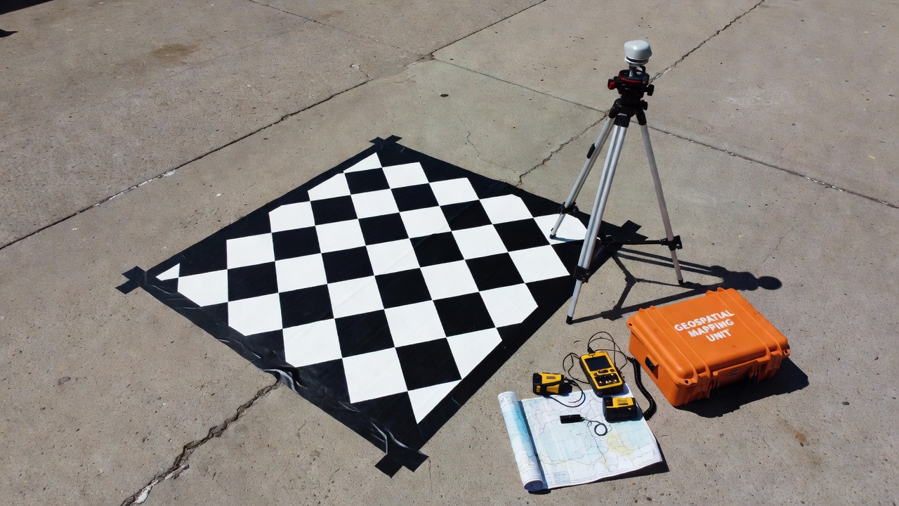
Ground Control Points (GCPs) are physically marked points on the ground with precisely surveyed coordinates, typically measured with GNSS receivers operating in RTK or static post-processing mode to achieve centimeter-level accuracy. GCPs are the primary mechanism for ensuring absolute accuracy — the degree to which the photogrammetric reconstruction matches real-world coordinates — as opposed to relative accuracy, which describes internal geometric consistency.
Each GCP consists of a visible target (typically a high-contrast black-and-white checkerboard pattern or cross) with dimensions of 30-60 cm for drone surveys at 5-10 cm GSD, or larger for higher-altitude flights. The target center is surveyed with accuracy better than the required final product accuracy — typically 1-2 cm horizontal and 2-3 cm vertical. GCP coordinates are referenced to a defined coordinate reference system (CRS), which for aviation and most infrastructure applications is WGS84 (ITRF) with appropriate projection for the local area.
GCP Distribution Strategy
The spatial distribution of GCPs significantly impacts the accuracy of the final reconstruction. Key principles for GCP placement include:
Perimeter placement: At least one GCP near each corner of the survey area constrains the overall geometry and prevents warping or “bowl” effects at the edges. For rectangular survey areas, a minimum of four perimeter GCPs is standard.
Interior distribution: Additional GCPs in the interior of the survey area improve accuracy, especially in areas of topographic variation. For surveys with elevation differences exceeding 10% of the flying height, GCPs should be placed at elevation extremes to control vertical accuracy.
Density guidelines: The ASPRS Positional Accuracy Standards for Digital Geospatial Data (2024 edition) and ISO 19157 provide guidance on GCP density. For 1:100 scale mapping (typical of infrastructure inspection), 1 GCP per 2-4 hectares is recommended, with a minimum of 5-8 GCPs per project regardless of area. Research consistently shows diminishing returns beyond 10-15 well-distributed GCPs for areas under 100 hectares.
Check Points and Independent Validation
Check points (CPs) are surveyed points with the same accuracy as GCPs but deliberately withheld from the photogrammetric processing. After the model is computed using GCPs, the coordinates of check points are extracted from the model and compared to their surveyed values. The differences — residuals — provide an independent accuracy assessment. Standards such as ASPRS 2024 and ICAO Annex 15 require reporting of accuracy based on check points, not GCPs, to avoid optimistic bias from using the same points for both control and validation.
Metric
Formula
Interpretation
RMSEₓ
√(Σ(Δx²)/n)
Root mean square error in X coordinate
RMSEᵧ
√(Σ(Δy²)/n)
Root mean square error in Y coordinate
RMSEz
√(Σ(Δz²)/n)
Root mean square error in Z coordinate
RMSEᵣ
√(RMSEₓ² + RMSEᵧ²)
Planimetric (horizontal) RMSE
CE90
1.7308 × RMSEᵣ
Circular error at 90% confidence (horizontal)
LE90
1.6449 × RMSEz
Linear error at 90% confidence (vertical)
For infrastructure inspection applications, typical accuracy requirements specified in ICAO Annex 14 and various national standards call for horizontal RMSE better than 3 cm and vertical RMSE better than 5 cm for precision pavement surveys. TarmacView’s photogrammetry-based inspection workflows routinely achieve these tolerances through optimized GCP networks and rigorous quality control procedures.
Photogrammetric Deliverables
Orthomosaic
An orthomosaic is a geometrically corrected, georeferenced composite image created by stitching together multiple aerial photographs. Unlike raw aerial images, which contain perspective distortions from camera tilt, lens optics, and terrain relief, an orthomosaic has been orthorectified — every pixel is projected to its correct planimetric position using the DSM and camera calibration data. The result is a seamless, true-to-scale image map where distances can be measured directly, just as on a traditional planimetric map.
Orthomosaics are produced at the native ground sample distance of the imagery, typically 0.5-3 cm for drone-based infrastructure surveys. Each pixel in the orthomosaic represents a known ground dimension, enabling direct measurement of linear features (crack lengths, pavement marking dimensions, joint spacing) and area computation (spalled zones, delaminated sections, standing water extent). The geometric accuracy of the orthomosaic is verified through check point analysis and reported as RMSE.
Digital Surface Model (DSM)
A Digital Surface Model (DSM) is a raster elevation model representing the earth’s surface including all features — buildings, vegetation, infrastructure, and terrain. In photogrammetry, the DSM is generated from the dense point cloud by interpolating elevation values onto a regular grid. The spatial resolution of the DSM typically matches the GSD of the source imagery, and the vertical accuracy follows the point cloud accuracy.
For infrastructure applications, the DSM enables:
Drainage analysis: Identification of ponding areas, low spots, and drainage path direction on pavement surfaces
Cross-slope measurement: Verification of pavement cross-slope against design specifications (typically 1.5-2.5% for runways per ICAO)
Longitudinal profile extraction: Measurement of pavement smoothness, grade changes, and vertical alignment
Cut/fill volume calculation: Quantification of material volumes for pavement rehabilitation projects
Dense Point Cloud
The dense point cloud is the primary 3D output of photogrammetric processing, containing millions to billions of georeferenced 3D points with associated color values from the source imagery. Each point has coordinates (X, Y, Z) and RGB color, enabling realistic visualization and precise measurement. Point clouds are typically exported in industry-standard formats including LAS, LAZ (compressed LAS), PLY, or XYZ text files.
Point density varies with survey parameters. At a 50 m flying height with a 20 MP camera, 70% forward overlap, and 70% side overlap, typical point densities of 500-2,000 points/m² are achieved. For close-range inspection of bridge components or building facades, densities can reach 10,000-100,000 points/m².
3D Mesh
A 3D mesh is a triangulated surface model derived from the dense point cloud, typically using Poisson surface reconstruction or Delaunay triangulation algorithms. The mesh represents the scanned surface as a continuous manifold of triangular faces, with texture applied from the source imagery for photorealistic visualization. Mesh models are essential for:
Visual inspection: Navigating a 3D model of a bridge, building, or pavement section to identify defects
Digital twin creation: Providing the geometric foundation for asset management systems
Finite element analysis: Converting mesh geometry to engineering analysis models
Virtual walkthroughs: Enabling remote inspection and stakeholder communication
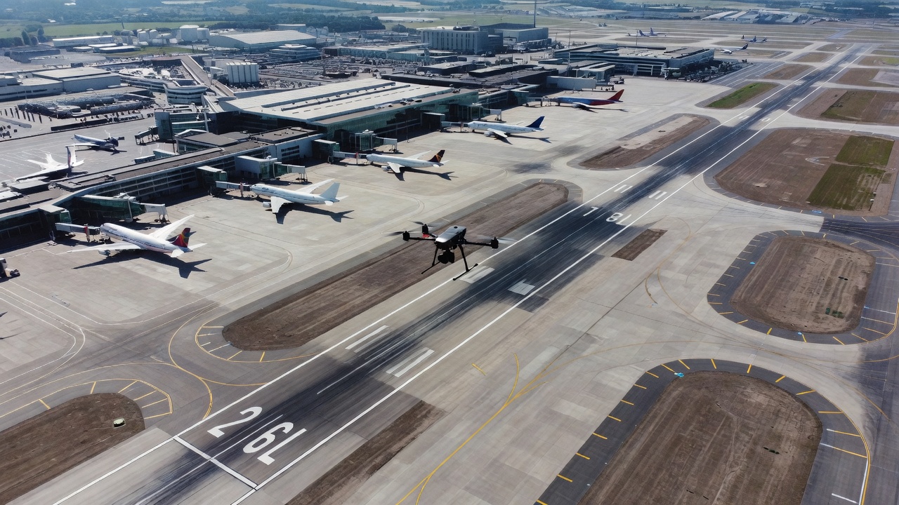
Drone Photogrammetry for Infrastructure Inspection
Drone-based photogrammetry has become the dominant method for infrastructure inspection across multiple sectors, offering significant advantages over traditional inspection methods. The combination of automated flight planning, high-resolution cameras, RTK/PPK GNSS positioning, and SfM photogrammetry processing enables rapid, comprehensive, and accurate condition documentation of large infrastructure assets.
Flight Planning for Infrastructure Surveys
Effective photogrammetric surveys require careful flight planning to ensure complete coverage, adequate overlap, and appropriate GSD. Key parameters include:
Flight altitude: Determines GSD (Ground Sample Distance). GSD = sensor pixel pitch × altitude / focal length. For a typical 20 MP camera with 24 mm focal length, flying at 50 m yields GSD = 1.1 cm/pixel. For crack detection where sub-millimeter cracks must be resolved, GSD should not exceed 2-3 mm/pixel, requiring flight altitudes of 15-30 m.
Overlap: Forward overlap of 80-90% and side overlap of 70-80% are standard for infrastructure surveys. Higher overlap increases processing time but improves reconstruction quality, especially for surfaces with limited texture (e.g., fresh concrete, asphalt).
Image acquisition: Nadir (vertical) images are standard for area mapping, but oblique images at 15-45° from vertical improve reconstruction of vertical surfaces such as bridge piers, building facades, and retaining walls. Some surveys combine nadir and oblique flights for complete 3D coverage.
RTK/PPK positioning: Drones equipped with RTK (Real-Time Kinematic) or PPK (Post-Processed Kinematic) GNSS record camera positions with 2-5 cm accuracy, significantly reducing the number of GCPs required. With RTK, absolute accuracy of 3-5 cm can be achieved with as few as 0-3 GCPs for well-structured surveys.
Applications in Infrastructure Inspection
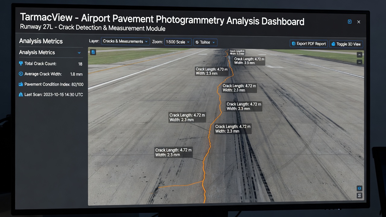
Pavement condition assessment: Photogrammetry enables automated detection and measurement of pavement distress including cracking (alligator, longitudinal, transverse, block), rutting, raveling, bleeding, and faulting. Crack widths of 0.5-3 mm can be reliably measured from orthomosaics with 1-2 mm GSD, enabling PCI (Pavement Condition Index) computation per ASTM D5340 for airfield pavements. TarmacView’s platform specializes in this application, integrating photogrammetric measurement with automated distress classification and PCI reporting.
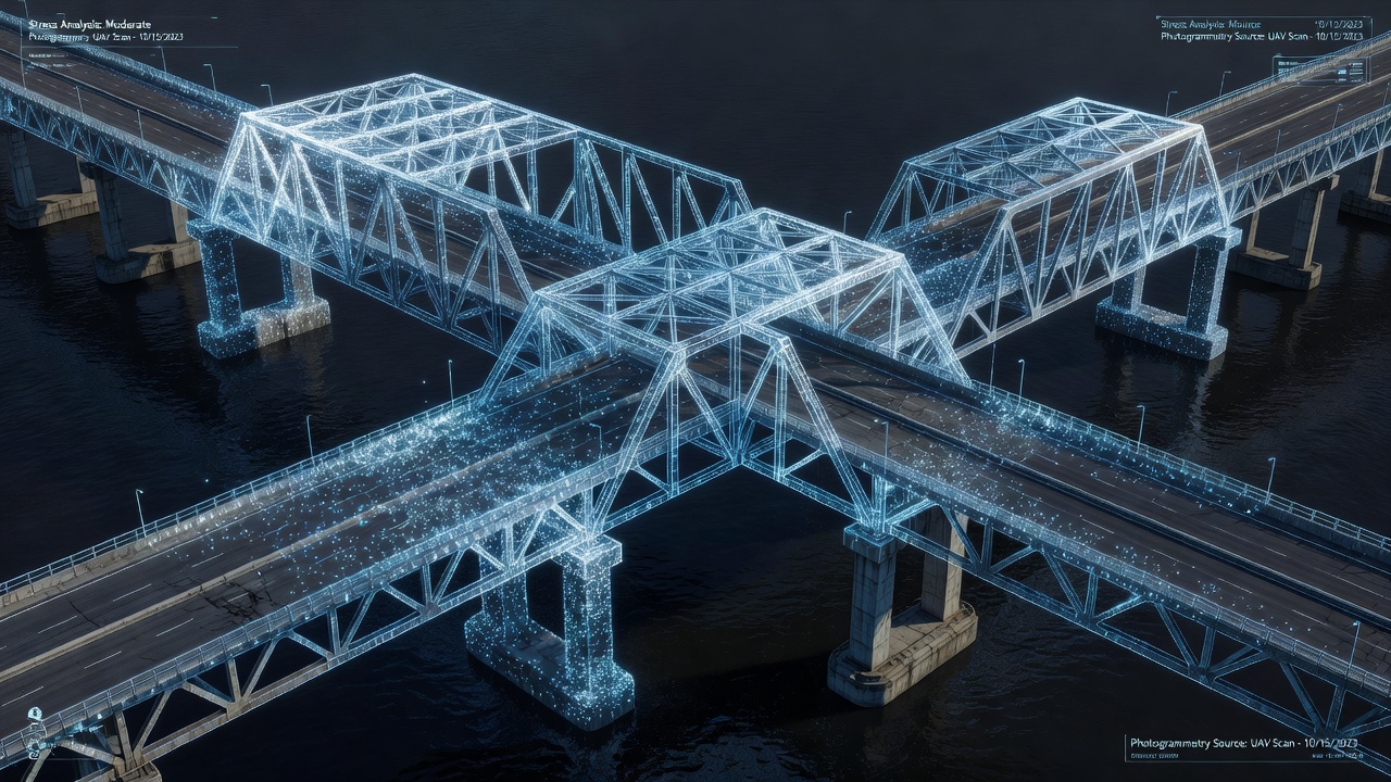
Bridge inspection: Close-range photogrammetry from drones provides comprehensive documentation of bridge components including deck surfaces, girders, bearings, abutments, and piers. Dense point clouds enable deflection measurement under load testing, crack mapping on concrete surfaces, corrosion assessment on steel components, and clearance verification. The FHWA and national bridge inspection standards increasingly recognize drone photogrammetry as an accepted inspection method for routine and in-depth inspections.
Building and facade inspection: Photogrammetric surveys of building exteriors detect façade cracking, spalling, efflorescence, moisture staining, and structural deformation. Thermal photogrammetry (using thermal cameras) extends inspection capability to subsurface moisture intrusion, insulation defects, and delamination.
Volume measurement: Stockpile volume calculation, excavation quantification, and erosion monitoring are standard photogrammetry applications. Volume accuracy of 1-3% is routinely achievable, validated against weighbridge measurements.
Change detection: Comparing sequential photogrammetric surveys of the same asset enables quantification of structural deformation, settlement, erosion, crack propagation, and construction progress. The detection threshold depends on survey accuracy: with 2 cm RMSE surveys, changes of 4-5 cm can be reliably detected at 95% confidence.
Infrastructure Asset
Typical GSD
Accuracy Achieved (with GCPs)
Key Measurements
Airport runway pavement
1-3 mm/pixel
2-5 mm horizontal, 3-8 mm vertical
Crack width, PCI, rut depth, cross-slope
Highway pavement
3-5 mm/pixel
5-10 mm horizontal, 8-15 mm vertical
IRI, crack mapping, shoulder condition
Bridge structure
2-5 mm/pixel
3-8 mm at 30 m range
Deflection, crack mapping, clearance
Building facade
3-10 mm/pixel
5-15 mm at 50 m range
Crack mapping, spalling, moisture zones
Earthworks/stockpiles
2-5 cm/pixel
3-5 cm horizontal, 5-10 cm vertical
Volume ±1-3%, cut/fill mapping
Accuracy Assessment and Quality Control
The Role of Check Points
Independent accuracy verification using check points is the gold standard for photogrammetric quality assurance. The process follows a strict protocol:
A minimum of 20 check points should be established for projects under 100 hectares (or 10% of the number of GCPs, whichever is larger), distributed across the survey area with emphasis on difficult terrain, edges, and areas critical to the project objectives.
Check point coordinates are measured in the field using survey-grade GNSS, with accuracy at least 3 times better than the expected photogrammetric accuracy.
After photogrammetric processing, the 3D coordinates of each check point are extracted from the point cloud or orthomosaic by a qualified analyst.
Residuals — the differences between surveyed and photogrammetric coordinates — are computed for each check point.
RMSE, CE90, and LE90 are computed and compared against the project accuracy requirements.
Standards and Compliance
The ASPRS Positional Accuracy Standards for Digital Geospatial Data (2024 edition) supersede earlier ASPRS and NSSDA standards. The standard defines accuracy classes tied to RMSE thresholds:
Accuracy Class
Horizontal RMSE (cm) at 1:100 scale
Vertical RMSE (cm)
ASPRS Class I
1.25
1.9
ASPRS Class II
2.5
3.8
ASPRS Class III
5.0
7.5
ASPRS Class IV
10.0
15.0
ASPRS Class V
25.0
37.5
For airfield pavement inspection, ICAO Annex 14 requirements for surface condition surveys typically correspond to ASPRS Class II or better, depending on the specific application. TarmacView’s inspection workflows target Class I-II accuracy for precision crack measurement and Class III for larger-area condition mapping.
Systematic Error Detection
Beyond RMSE, quality control must address systematic errors that may not appear in RMSE statistics. Systematic error detection methods include:
Residual plotting: Plotting check point residuals against X, Y, and Z coordinates to identify spatial trends (e.g., increasing error toward edges)
Temporal analysis: For repeat surveys, plotting residuals against time or survey parameters to detect drift or seasonal effects
Cross-validation: Splitting GCPs into multiple subsets and comparing reconstructions to assess robustness
Photogrammetry-Based Measurement Capabilities
Crack Width Measurement
Precision crack measurement from photogrammetric data requires sub-pixel measurement techniques. The extracted sub-pixel edge detection method fits the edge response function across a crack feature to determine its boundaries with precision of 0.1-0.2 pixels. For a GSD of 1 mm/pixel, this translates to crack width measurements with 0.1-0.2 mm precision. Validation studies on airport pavements demonstrate that photogrammetric crack width measurements agree with manual micrometer measurements within ±0.3 mm for cracks 0.5-10 mm wide.
TarmacView’s automated crack detection pipeline integrates photogrammetric orthomosaics with deep learning segmentation models (typically based on U-Net or DeepLab architectures) trained on thousands of labeled pavement distress images. Detected cracks are vectorized, measured, and classified by type, width, and severity according to ASTM D5340 and ICAO pavement evaluation guidelines.
Area and Volume Measurement
Area measurement from orthomosaics is fundamentally accurate because the orthomosaic is a true-scale, distortion-free representation of the ground surface. The accuracy of area measurement depends on the accuracy of the boundary delineation, which is typically within 2-3 pixels. For pavement distress areas (spalling, patching, raveling), area accuracy of 95-98% is routinely achievable.
Volume measurement requires a DSM or point cloud of the surface before and after change, or a pre-existing reference surface. The volume between two surfaces is computed by subtracting elevation values at each grid cell and summing the product of height difference and cell area. For stockpile volume measurement, accuracy of 1-3% against weighbridge validation is standard. For pavement milling or overlay volume, accuracy of 2-5% is typical depending on surface texture and survey quality.
Deformation Monitoring
Repeated photogrammetric surveys of the same asset enable deformation monitoring through direct comparison of point clouds or DSMs. The Cloud-to-Cloud (C2C) distance method computes nearest-neighbor distances between two point clouds. The Multiscale Model-to-Model Cloud Comparison (M3C2) algorithm provides statistically rigorous distance computation with confidence intervals, accounting for point cloud uncertainty and surface roughness.
For bridge deflection monitoring, photogrammetric measurements under static load typically achieve precision of 2-5 mm at ranges of 20-50 m, competitive with traditional dial gauges and total station measurements. Dynamic deflection monitoring remains challenging for photogrammetry due to the synchronization requirements between multiple cameras, though stereo photogrammetry systems have demonstrated 1 mm precision at 100 Hz for laboratory tests.
Integration with Inspection Workflows
End-to-End Inspection Pipeline
Photogrammetry integrates into infrastructure inspection workflows through a structured pipeline:
Phase 1 — Planning: Define inspection objectives, required accuracy, asset characteristics, and site constraints. Select camera sensor, flying altitude, overlap parameters, and GCP network design. Obtain flight permissions and airspace coordination where required.
Phase 2 — Field Acquisition: Deploy and survey GCPs. Execute automated flight mission with programmed waypoints, overlap, and camera trigger intervals. For infrastructure inspection, inspect imagery quality in the field to ensure focus, exposure, and coverage are adequate.
Phase 3 — Photogrammetric Processing: Transfer images to processing software. Perform quality check on image metadata and GNSS logs. Execute SfM processing: feature extraction, matching, sparse reconstruction, GCP identification and marking, bundle adjustment, dense reconstruction, DSM/orthomosaic generation. Validate accuracy using check points. For large projects, processing a 300-image survey at 20 MP takes approximately 4-8 hours on a modern workstation with GPU acceleration.
Phase 4 — Analysis and Measurement: Import orthomosaic, DSM, and point cloud into analysis software. Perform distress detection (automated or manual), crack measurement, area computation, volume calculation, or deformation analysis. Generate inspection reports with measurements, images, and accuracy statements.
Phase 5 — Archival and Monitoring: Store photogrammetric data with metadata including date, accuracy, coordinate reference system, and sensor parameters. Compare with historical surveys for change detection. Update asset management systems with inspection results.
Regulatory Frameworks for Photogrammetric Inspection
Several international and national standards govern the use of photogrammetry for infrastructure inspection:
ICAO Annex 14 — Aerodromes: Specifies geometric standards for runway surfaces, including longitudinal slope, transverse slope, and surface condition. ICAO Doc 9157 (Aerodrome Design Manual) provides guidance on survey methods including photogrammetry for pavement evaluation.
ICAO Annex 15 — Aeronautical Information Services: Establishes quality requirements for aeronautical data including survey data, requiring accuracy levels commensurate with the criticality of the data.
ICAO Annex 6, Part IV — RPAS Operations: Governs drone operations for inspection missions, requiring operator certification, remote pilot licensing, and airworthiness compliance for international operations per Annex 6 Part IV and ICAO Doc 10019.
ISO/TS 19159-1:2014: Specifies calibration procedures for optical sensors used in mapping and inspection applications, including laboratory, in-situ, and test-site calibration methods.
ISO 19130-1:2018 — Imagery Sensor Models for Geopositioning: Defines the framework for sensor models relating image coordinates to geographic coordinates, essential for photogrammetric processing software interoperability.
ISO 19157 — Data Quality: Establishes principles for reporting data quality in geographic information, including completeness, logical consistency, positional accuracy, temporal accuracy, and thematic accuracy.
Photogrammetry Software Tools
Commercial Solutions
Agisoft Metashape is widely regarded as the industry standard for drone photogrammetry, offering comprehensive processing from image alignment through dense reconstruction, DSM/orthomosaic generation, and measurement. It supports Python scripting for workflow automation, making it popular for infrastructure inspection pipelines. Metashape handles projects from small object-scale to large area surveys (10,000+ images) through its network processing capability.
Pix4Dmapper provides an integrated photogrammetry solution specifically optimized for drone surveys, with automated quality reporting, GCP management, and accuracy assessment. Pix4Dmatic extends processing to very large projects. The Pix4D ecosystem includes specialized modules for agriculture, construction, and inspection.
RealityCapture (by Epic Games/Capturing Reality) is known for its exceptional processing speed and quality, particularly for close-range photogrammetry of structures and objects. It is widely used in the digital twin and heritage documentation sectors. Its GPU-accelerated processing pipeline is among the fastest available.
Bentley ContextCapture is the leading solution for large-scale infrastructure photogrammetry, integrating with Bentley’s broader digital twin and BIM ecosystem. It is widely used in transportation, energy, and civil engineering applications.
Open-Source Solutions
OpenDroneMap (ODM) is the most prominent open-source photogrammetry platform, providing full SfM and MVS processing pipelines. It supports command-line and web interface operation, making it suitable for automated processing pipelines. The quality and accuracy of ODM have improved significantly and now approach commercial software levels for many applications.
Meshroom (by AliceVision) is an open-source photogrammetry framework with a node-based graphical interface, making it accessible for research and education while supporting advanced features including HDR reconstruction and depth map fusion.
COLMAP is a general-purpose SfM and MVS library widely used in computer vision research, offering state-of-the-art feature matching and reconstruction quality. It is command-line driven and commonly integrated into custom processing pipelines.
TarmacView Integration
TarmacView’s inspection platform integrates photogrammetric principles at its core, processing drone imagery of airport pavements to produce precision orthomosaics at 1-3 mm GSD with verified accuracy. The platform automates crack detection and measurement using computer vision and deep learning, computes Pavement Condition Index per ASTM D5340, tracks changes through temporal comparison of successive surveys, and generates ICAO-compliant inspection reports. By combining photogrammetric accuracy with automated distress analysis, TarmacView enables infrastructure managers to move from subjective visual inspection to objective, measurable, data-driven pavement condition assessment.
References
American Society for Photogrammetry and Remote Sensing (ASPRS). Positional Accuracy Standards for Digital Geospatial Data. 2024 Edition.
International Civil Aviation Organization. Annex 14 — Aerodromes, Volume I: Aerodrome Design and Operations. 8th Edition, 2018.
International Civil Aviation Organization. Doc 9157 — Aerodrome Design Manual, Part 3: Pavements. 2nd Edition, 2002.
International Civil Aviation Organization. Doc 10019 — Manual on Remotely Piloted Aircraft Systems (RPAS). 2015.
International Organization for Standardization. ISO/TS 19159-1:2014 — Geographic Information — Calibration and Validation of Remote Sensing Imagery Sensors and Data — Part 1: Optical Sensors.
International Organization for Standardization. ISO 19130-1:2018 — Geographic Information — Imagery Sensor Models for Geopositioning — Part 1: Fundamentals.
International Organization for Standardization. ISO 19157:2013 — Geographic Information — Data Quality.
Luhmann, T., Robson, S., Kyle, S., & Boehm, J. Close-Range Photogrammetry and 3D Imaging. 3rd Edition, De Gruyter, 2019.
ASTM D5340-19. Standard Test Method for Airport Pavement Condition Index Surveys.
Federal Highway Administration. Bridge Inspection Practices Using Unmanned Aerial Systems. FHWA-HIF-19-002, 2019.
Frequently Asked Questions
Photogrammetry is the science of making measurements from photographs. It works by capturing overlapping images of an object or area from different positions, then using triangulation to calculate 3D coordinates. Software identifies common points (tie points) across overlapping images, traces light rays back to their origins using the collinearity condition, and solves for 3D positions through bundle adjustment. The output includes point clouds, digital surface models, orthomosaics, and 3D meshes accurate to centimeter or even millimeter levels.
Photogrammetry uses passive optical sensors (cameras) and relies on natural light and image texture to reconstruct 3D geometry. LiDAR is an active sensor that emits laser pulses and measures return times to directly measure distances. Photogrammetry excels at visual texture, color information, and cost-effective large-area coverage. LiDAR penetrates vegetation, works in darkness, and produces accurate point clouds even on low-texture surfaces. Many projects combine both for optimal results.
With proper ground control points (GCPs) and RTK/PPK GNSS, drone photogrammetry routinely achieves 1-3 cm horizontal accuracy and 2-5 cm vertical accuracy relative to the GCP network. Without GCPs, accuracy typically degrades to 2-5 m horizontally and 5-20 m vertically depending on the drone's onboard GNSS quality. Accuracy is verified using independent check points and reported as RMSE per standards like ASPRS Positional Accuracy Standards.
Professional aerial photogrammetry requires 70-90% forward overlap and 60-80% side overlap between images. This ensures every point on the ground appears in at least 3-5 images for robust triangulation. For close-range photogrammetry of structures, 80% overlap in both directions is standard. The exact number depends on the area size, ground sample distance (GSD), camera specifications, and scene complexity.
Structure from Motion (SfM) is a computer vision technique that simultaneously solves for camera positions, orientations, and 3D scene geometry from a set of overlapping images. Unlike classical photogrammetry that requires known camera positions and GCPs upfront, SfM automatically estimates camera parameters and sparse 3D points from image feature matches alone. It then refines everything through bundle adjustment. SfM has revolutionized drone photogrammetry by enabling fully automated 3D reconstruction from unpositioned image sets.
The primary deliverables include: (1) Orthomosaic — a geometrically corrected, georeferenced 2D image map with uniform scale; (2) Digital Surface Model (DSM) — a 3D elevation model capturing all surface features including vegetation and structures; (3) Digital Terrain Model (DTM) — a bare-earth elevation model with vegetation and structures removed; (4) Dense Point Cloud — millions or billions of 3D points representing the scanned surface; (5) 3D Mesh — a triangulated surface model for visualization and analysis; and (6) Contour Lines — elevation isolines derived from the DSM or DTM.
Photogrammetry enables non-contact measurement and documentation of infrastructure condition. Applications include: pavement crack detection and width measurement on runways and roads; bridge deflection monitoring and deformation analysis; volume calculation of stockpiles, excavations, and erosion; surface deterioration mapping of concrete and asphalt; as-built verification against design models; historical change detection through temporal comparison of repeated surveys; and digital twin creation for asset management systems.
Industry-leading photogrammetry software includes Agisoft Metashape, Pix4Dmapper, Bentley ContextCapture, RealityCapture (Capturing Reality), 3DF Zephyr, DroneDeploy, and OpenDroneMap (open-source). For close-range and object photogrammetry, solutions include RealityCapture, Meshroom (open-source), and Autodesk ReCap. These tools handle image alignment, dense reconstruction, mesh generation, orthomosaic production, and measurement extraction. TarmacView integrates photogrammetric principles specifically for airport pavement inspection and runway condition analysis.
Advanced Photogrammetry for Infrastructure
Harness drone-based photogrammetry for precise infrastructure inspection, pavement analysis, and 3D mapping. Our platform delivers survey-grade accuracy from aerial imagery with automated crack detection, volume calculation, and change analysis.
A point cloud is a set of 3D data points representing the external surfaces of objects or terrain, generated by LiDAR scanning or photogrammetry. In infrastruct...
A comprehensive glossary and guide to surveying, measurement, and mapping—covering definitions, advanced concepts, ICAO/international standards, professional ro...
LiDAR (Light Detection And Ranging) is an active remote sensing technology that emits laser pulses and measures their return time to create dense, accurate 3D p...
28 min read
Surveying
Remote Sensing
+6
Cookie Consent We use cookies to enhance your browsing experience and analyze our traffic. See our privacy policy.