Point Cloud (Set of Data Points in Three-Dimensional Space) — Surveying

Definition: What Is a Point Cloud?

A point cloud is a digital collection of spatially defined points in three-dimensional (3D) space, each represented by X, Y, and Z coordinates. These points collectively form a highly detailed numerical representation of real-world surfaces, objects, or entire environments. Often, each point can also store additional information such as color (RGB), intensity, classification (e.g., ground, vegetation), and timestamps. Unlike traditional CAD models, point clouds do not connect points with surfaces, but provide a dense, raw dataset that captures physical geometry with great fidelity.

Point clouds are fundamental in modern surveying, mapping, and engineering. Their strength lies in bridging the physical and digital worlds—providing highly accurate, measurable digital twins of real-world conditions. Surveyors use point clouds for topographic mapping, infrastructure documentation, and as the foundation for 3D models, digital elevation models (DEMs), and Building Information Modeling (BIM). As sensor technology advances, point clouds grow ever denser and more precise, making them indispensable for applications ranging from construction, asset management, and environmental analysis to immersive visualization in virtual and augmented reality.

How Point Clouds Are Generated

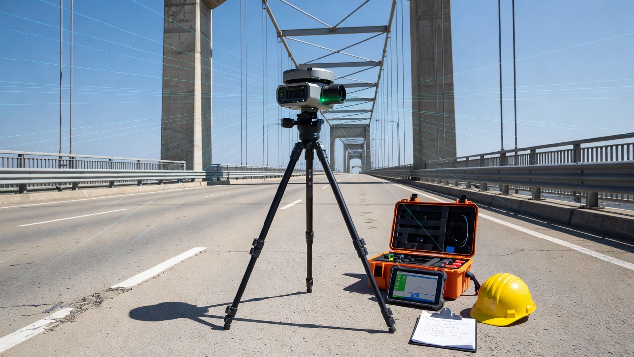
LiDAR (Light Detection and Ranging)

LiDAR is the most widely used technology for point cloud generation in surveying. It emits rapid laser pulses toward surfaces and measures the time it takes for each pulse to return. Using precise orientation data (from GPS and inertial units), each detected pulse is mapped to an X, Y, Z coordinate. Terrestrial, mobile, and airborne LiDAR systems can capture millions of points per second, achieving sub-centimeter accuracy for detailed surveys.

Terrestrial LiDAR is ideal for scanning building interiors and structural details. Airborne LiDAR is used for mapping terrain, forests, and large infrastructure, and can even penetrate vegetation to capture bare earth. LiDAR point clouds often include intensity (signal return strength) and multi-return data (recording reflections from multiple surfaces), which enhances analysis, such as distinguishing between ground and vegetation.

Photogrammetry

Photogrammetry reconstructs 3D geometry from overlapping photographs. By identifying common features across multiple images and triangulating their position, software calculates the spatial coordinates of millions of points. Photogrammetry is widely used in aerial mapping (with drones or manned aircraft) and also for capturing facades or archaeological sites.

Photogrammetry’s main advantage is its ability to generate colorized point clouds, as each point can inherit RGB values from photographs. With high-quality images and accurate ground control points (GCPs), photogrammetry can achieve survey-grade results. However, it may be less effective in low-light or featureless environments.

Other Methods

Other technologies used for point cloud creation include:

• Structured Light Scanning: Projects patterns onto a surface and uses cameras to reconstruct 3D geometry—ideal for industrial inspection and reverse engineering.
• Radar/Sonar: Used for subsurface (ground-penetrating radar) or underwater (sonar) mapping.
• Depth Cameras: Infrared or time-of-flight sensors (e.g., Microsoft Kinect) for real-time 3D capture in robotics and indoor mapping.

Each method has specific strengths depending on accuracy requirements, environment, and application.

Structure and Characteristics of Point Cloud Data

Attributes of Points

Each point in a point cloud typically contains:

• X, Y, Z coordinates: The spatial position in a defined coordinate system.
• Color (RGB): Captured via photogrammetry or color LiDAR.
• Intensity: Strength of LiDAR return, useful for material identification.
• Classification: Labels such as ground, building, or vegetation.
• Timestamp: For mobile/kinematic mapping and change monitoring.
• Return Number: Identifies if the point is from the first, last, or intermediate LiDAR pulse return.

These attributes enable advanced analysis, feature extraction, and regulatory compliance.

Density, Resolution, and Accuracy

• Density: Number of points per square meter. Terrestrial LiDAR can exceed 1,000 pts/m², airborne LiDAR typically ranges from 2–20 pts/m².
• Resolution: The minimum feature size detectable, tied to point spacing.
• Accuracy: Determined by sensor technology, ground control, and processing. Standards like ICAO’s and ASPRS’s specify required tolerances for survey data.

Point Cloud Types

• Ordered (Regular): Grid or matrix-based, from structured light or certain scanners.
• Unordered (Irregular): Typical of LiDAR/photogrammetry, points are scattered based on scene geometry.
• Colorized: Points include RGB for visualization.
• Classified: Semantic labels (e.g., ground, building) applied.
• Time-Stamped: For dynamic/moving scenes.

Data Formats

Standardized formats ensure interoperability across GIS, CAD, and BIM environments.

Applications of Point Clouds

Topographic and Land Surveys

Point clouds are used to create digital terrain models (DTMs), digital surface models (DSMs), and contour maps. Airborne LiDAR enables rapid, high-density mapping for flood risk assessment, land development, and environmental monitoring. Volumetric calculations (e.g., cut-and-fill in earthworks) and site boundary surveys also benefit from point clouds.

Building and Infrastructure Surveys

Terrestrial scanning generates highly detailed as-built documentation and underpins 2D drawings, 3D models, and BIM integration. Infrastructure surveys (bridges, tunnels, roads) use point clouds for renovation planning, safety assessments, and asset management. Mobile LiDAR systems can scan railways and roads at speed for maintenance and compliance.

Construction Monitoring and Quality Control

Regular scanning during construction allows progress monitoring, deviation analysis, and clash detection. Comparing as-built point clouds to design models identifies discrepancies early, reducing rework and cost overruns. Permanent digital records aid documentation and dispute resolution.

Heritage and Cultural Documentation

Non-contact scanning preserves fragile heritage sites and archaeological remains. Detailed point clouds support restoration, virtual tourism, and disaster recovery. International bodies (ICOMOS, UNESCO) endorse point cloud documentation for cultural heritage preservation.

Industrial and Plant Surveys

Point clouds enable comprehensive digital twins of factories, refineries, and process plants. They support asset management, maintenance, reverse engineering, and safety assessments—improving operational efficiency and minimizing downtime.

Environmental and Geospatial Analysis

Airborne LiDAR penetrates vegetation, capturing ground and canopy structure for forestry, flood modeling, and climate studies. Point clouds support landscape change monitoring, erosion analysis, and ecosystem research.

Integration and Workflow

Modern surveying integrates point clouds with:

• GIS: Advanced spatial analysis, mapping, and change detection.
• CAD/BIM: Extraction of models, clash detection, and digital twin creation.
• Asset Management: Ongoing facility and infrastructure maintenance.
• Regulatory Compliance: Meeting standards for aerodrome, obstacle, and infrastructure surveys.

Software such as CloudCompare, Autodesk ReCap, Bentley ContextCapture, and open libraries (PDAL, PCL) enable visualization, conversion, analysis, and integration of point clouds across disciplines.

Summary

Point clouds are revolutionizing surveying, engineering, and geospatial sciences. They provide the raw, accurate, and richly attributed data needed for detailed 3D modeling, digital twins, and spatial analysis. As technologies like LiDAR and photogrammetry evolve, point clouds will continue to drive innovation in mapping, construction, asset management, and environmental monitoring.