Inertial Profiler
A vehicle-mounted inertial profiler uses laser height sensors and accelerometers to measure longitudinal pavement profile at highway speeds, computing IRI and r...
27 min read
Pavement Testing
Pavement Smoothness
+2
A profilograph is a low-speed rolling straightedge device that measures longitudinal pavement profile deviations to assess smoothness. California and Rainhart profilographs produce graphical traces used to compute Profile Index (PrI) for construction acceptance of new asphalt and concrete pavements.
A profilograph is a contact-type, low-speed pavement profiling device used to measure the longitudinal smoothness (or roughness) of newly constructed asphalt and concrete pavements. Also known as a rolling straightedge, the profilograph consists of a rigid truss frame supported by multiple wheels at each end with a center profiling wheel that records vertical deviations of the pavement surface from a moving reference plane. The device produces a continuous graphical record called a profilogram or profilograph trace, which is analyzed to compute the Profile Index (PrI) — a statistical quantification of pavement smoothness expressed in inches per mile or millimeters per kilometer. Profilographs have been the primary tool for construction quality control and acceptance testing of pavement smoothness since their introduction in the 1940s, though they are increasingly being supplemented or replaced by inertial profilers in many jurisdictions.
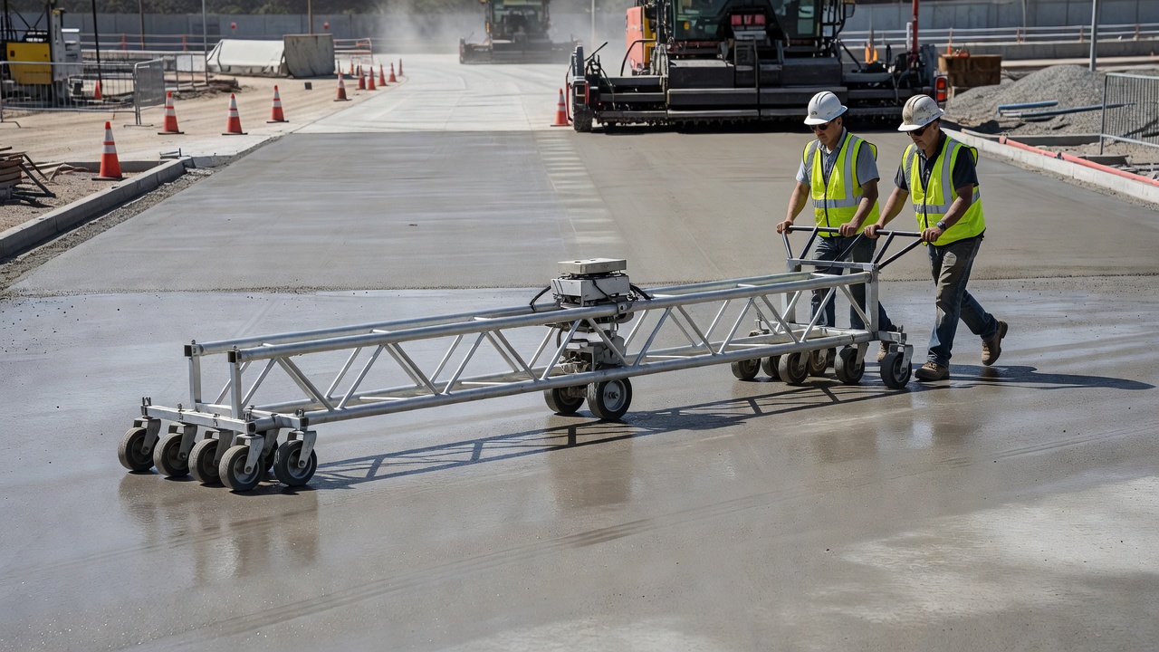
The profilograph is defined by ASTM E1274 as an apparatus that measures pavement roughness by recording the deviations of a pavement surface from a moving reference plane established by the profilograph’s support wheels. The fundamental principle of operation is that the device creates a datum line between the front and rear support wheel groups, and the center wheel, located at the midpoint of the 25-foot (7.6-meter) wheelbase, measures the vertical displacement of the pavement surface relative to that datum. These vertical measurements are recorded continuously as the device is propelled along the pavement at walking speed, producing a scaled graphical representation of the pavement profile.
The primary purpose of profilograph testing is construction quality control and acceptance. Pavement smoothness is one of the most important indicators of construction quality from the road user’s perspective. Numerous surveys have demonstrated that pavement smoothness is the single most important factor in how the traveling public rates highway quality. Beyond user satisfaction, smooth pavements provide measurable benefits including improved fuel economy (rough pavements can increase fuel consumption by 2% to 5%), reduced vehicle maintenance costs, extended pavement service life, improved safety through better tire contact, and reduced dynamic loading on the pavement structure. The profilograph’s role is to provide a quantitative, reproducible measure of initial smoothness that can be compared against specification limits for construction acceptance, and to identify localized areas of roughness (must grinds) that require correction before the pavement is opened to traffic.
ASTM E867 defines pavement roughness as “the deviations of a pavement surface from a true planar surface with characteristic dimensions that affect vehicle dynamics, ride quality, dynamic pavement loading, and drainage.” The profilograph measures a subset of these deviations, specifically those with wavelengths between approximately 1 foot and 75 feet (0.3 to 23 meters), which encompasses the range most relevant to ride quality for passenger vehicles.
The California profilograph, also called the California-type profilograph or Hveem profilograph, is the most widely used profilograph design in the United States. It was invented by Francis Hveem and first constructed in 1940 by the Materials and Research Division of the California Division of Highways (now Caltrans). The device was developed to provide a more objective and reproducible measure of pavement smoothness than the manual straightedge method that was standard practice at the time.
The California profilograph consists of a lightweight aluminum truss structure 25 feet (7.6 meters) long that can be disassembled into three or more sections for transport. The truss sections connect using quick-acting clamps and are match-marked to ensure correct reassembly. The truss supports a system of wheels at each end — typically four wheels on one side and two on the other in a staggered configuration — that establish the reference datum. A center profiling wheel is linked mechanically or electronically to a recording mechanism. On the original mechanical profilographs, the center wheel was connected via a control cable to a pen that traced the profile on a strip chart recorder driven by a distance-measuring wheel through a chain and gearbox assembly. The recording chart has a longitudinal scale of 1:300 (1 inch on the chart equals 25 feet on the pavement) and a vertical scale of 1:1 (true scale), meaning that vertical deviations are recorded at actual size while the horizontal distance is compressed 300 times.
The operating procedure for the California profilograph requires a crew of two people. The device is propelled at walking speed (approximately 3 mph or 5 km/h) by manual pushing or by a suitable propulsion unit such as a garden tractor. The operator must maintain the profiling wheel in the specified wheelpath using a pointer attached to the profilograph. Testing from header to header (between transverse construction joints) is standard practice for concrete pavements. The device can measure approximately 3 to 5 kilometers (1.9 to 3.1 miles) of pavement per hour under favorable conditions.
Caltrans developed California Test Method 526 (CTM 526) which standardizes the procedure for operating the profilograph and reducing the trace to obtain the Profile Index. This test method specifies the blanking band width (traditionally 0.2 inches or 5 mm, and increasingly the zero blanking band), the minimum scallop height and length to be counted (0.03 inches or 0.7 mm vertical and 2 feet or 0.6 m longitudinal), and the method for calculating PI. Many other state highway agencies have adopted similar procedures based on CTM 526.
A critical design feature of the California profilograph is its wheel configuration. The support wheels are arranged in a staggered pattern so that no two wheels cross the same bump or depression at the same time. This arrangement averages out short-wavelength surface texture and minor irregularities, allowing the device to respond primarily to profile features that affect ride quality. However, because the front and rear wheels are in constant contact with the pavement surface, the profilograph cannot accurately measure the true pavement profile. The device’s response is a function of both the actual pavement profile and the interaction of the wheel systems with that profile. Research by Kulakowski and Wambold demonstrated that the California profilograph correctly measures some wavelengths, amplifies others by up to a factor of two (particularly in the 20- to 40-foot wavelength range), and attenuates wavelengths between 10 and 15 feet. This non-linear frequency response means that the profilograph trace is not a true elevation profile but rather a filtered representation that biases certain wavelength ranges.
Most profilographs in use today are computerized systems that replace the mechanical strip chart recorder with electronic sensors and data acquisition hardware. The center wheel is connected to a rotational encoder or linear variable differential transformer (LVDT) that converts vertical displacement into an electronic signal. A distance-measuring encoder on the profiling wheel or a separate distance wheel provides longitudinal position data. The computer records the profile at regular distance intervals (typically every 1 inch or 25 mm) and can compute the Profile Index automatically using built-in software implementing the blanking band algorithm. Computerized profilographs eliminate the need for manual trace reduction, reduce operator variability, and provide immediate results in the field. They also store the raw profile data, which can be reprocessed with different blanking band settings or exported to analysis software such as ProVAL for further evaluation.
The Rainhart profilograph is an alternative design that differs mechanically from the California type. Where the California profilograph uses a 25-foot (7.6-meter) frame with support wheels concentrated at the ends, the Rainhart device uses a 24.75-foot (7.5-meter) frame with twelve support wheels evenly spaced along the frame at offsets up to 22 inches (560 mm). The key difference is that on the Rainhart profilograph, no wheel follows the same path — each wheel tracks a unique line on the pavement surface. This staggered wheel arrangement establishes the reference datum over the entire length of the unit and over a width of 44 inches (1,118 mm), rather than only at the ends as with the California type. In theory, the Rainhart configuration provides better averaging of pavement texture and minor irregularities, resulting in a more stable reference datum. Both types produce similar profilograph traces and are used to compute Profile Index using the same blanking band methodology. The choice between California and Rainhart profilographs is primarily a matter of agency preference and historical practice.
For mechanical profilographs that produce strip chart output, the trace must be reduced manually to determine the Profile Index. Manual trace reduction is a skilled task requiring careful technique. The procedure, as specified in California Test Method 526 and similar protocols, involves several distinct steps:
Step 1 — Outline Trace: Using a red or contrasting color ballpoint pen, the technician traces through the middle of the spikes on the original profilogram. This outlining process averages out spikes and minor deviations caused by rocks, dirt, pavement surface texture, or transverse grooving. The purpose is to create a smooth trace that represents the actual pavement profile without the noise introduced by surface texture. Outlining was adopted by many agencies to reduce variability between technicians and expedite the reduction process. Modern computerized systems perform this filtering mathematically.
Step 2 — Position Blanking Band: The blanking band scale is placed over the outlined profile trace with the dashed reference line as nearly centered on the trace as possible. The blanking band is a plastic scale 40 mm (1.6 inches) wide and 333 mm (13.1 inches) long, representing 0.1 km (0.06 miles or 528 feet) of pavement at the 1:300 longitudinal scale. At the center of the scale is an opaque band 5 mm (0.2 inches) wide extending the full length. Parallel scribed lines at 2 mm (0.08 inch) intervals flank the center band on both sides. The blanking band is positioned so that the opaque center band blanks out as much of the profile trace as possible, with deviations above and below the band approximately balanced. For superelevated curves where the trace shifts, the profile is broken into short sections and the blanking band is repositioned on each section.
Step 3 — Compute Profile Index: Starting from one end of the scale, the heights of all scallops (deviations or excursions) appearing both above and below the blanking band are measured to the nearest 1 mm (0.04 inch) and totaled. Scallops are only counted if they project 0.6 mm (0.03 inch) or more vertically and extend longitudinally for 0.6 m (2 feet or 0.08 inch on the profilogram) or more. Double-peaked scallops are counted only once at the highest peak. The sum of recorded heights within the 0.1-mile segment is the Profile Index for that segment, expressed in inches per mile or mm per km. The process is repeated for each 0.1-mile segment along the pavement.
Step 4 — Identify Must Grinds: The technician identifies localized bumps or dips exceeding the specified threshold (typically 0.3 inches deviation in 25 feet for Caltrans specifications). Using a bump template — a plastic template with a slot or edge parallel to a 1-inch (25-foot) marked length — the technician draws a chord across each prominent peak or valley. Any portion of the trace extending above or below this chord indicates a bump or dip requiring correction. The station location of each must grind is recorded for the grinding crew.
The Profile Index (PrI) — also designated as PI — is a statistical measure of pavement smoothness derived from the profilograph trace. It represents the accumulated vertical deviation of the pavement profile from the established reference line, normalized per unit length of pavement. The units of measurement are inches per mile (in/mi) in the United States customary system and millimeters per kilometer (mm/km) in SI units. The conversion factor is 1 in/mi = 15.78 mm/km.
The mathematical basis of the Profile Index is deceptively simple: the sum of all scallop heights exceeding the blanking band width within a measured segment, divided by the length of that segment, scaled to the standard unit distance. In equation form:
PrI (in/mi) = (Total measured scallop heights in inches) ÷ (Segment length in miles)
For the typical 0.1-mile (528-foot) segment, the measured scallop heights in inches are multiplied by 10 to obtain inches per mile.
The blanking band width has a profound effect on the calculated PI value. The 0.2-inch blanking band has been the traditional standard since the early days of profilograph testing. This 5 mm wide opaque band hides minor deviations from the count, meaning that only profile features exceeding 0.2 inches in amplitude are included in the PI calculation. The resulting PI values are relatively low, with typical acceptance limits of 7 to 10 in/mi for highway pavements. Many agencies have transitioned to the zero blanking band, which uses only a thin reference line and captures all profile deviations regardless of amplitude. Zero blanking band PI values are typically 3 to 5 times higher than 0.2-inch blanking band values for the same pavement, with acceptance limits commonly in the range of 20 to 45 in/mi.
The relationship between 0.2-inch blanking band PI and zero blanking band PI is not linear and depends on the specific characteristics of the pavement profile. Agencies transitioning from one blanking band to another typically conduct correlation studies to establish conversion factors for their specific conditions. The FHWA publication Achieving a High Level of Smoothness in Concrete Pavements Without Sacrificing Long-Term Performance (FHWA-HRT-05-068) provides guidance on this relationship.
The International Roughness Index (IRI) is a standardized measure of pavement roughness developed by the World Bank in a landmark 1982 study (the International Road Roughness Experiment) to establish a correlation and calibration standard for roughness measurements worldwide. IRI is defined mathematically as a property of the true longitudinal profile of the pavement, and therefore can be computed from profile measurements obtained with any valid profiling device — profilograph, inertial profiler, Dipstick, rod and level, or walking profiler — provided the raw elevation profile data is available.
The IRI computation is based on the quarter-car model, a mathematical simulation of one corner of a passenger vehicle traversing the measured profile at 80 km/h (50 mph). The quarter-car model consists of four components: a tire represented as a vertical spring with a specific spring constant, the unsprung mass (axle and wheel assembly), a suspension spring and damper (shock absorber), and the sprung mass (one-quarter of the vehicle body weight). As the simulated tire follows the pavement profile, the mathematical model calculates the relative motion between the sprung and unsprung masses — essentially, the suspension deflection — at each point along the profile. The absolute values of all suspension deflections are summed over the measured length and divided by that length to obtain the average suspension motion. This accumulated suspension travel per unit distance, expressed in meters per kilometer (m/km) or inches per mile (in/mi), is the IRI value.
The IRI filter has maximum sensitivity to pavement wavelengths of approximately 8 feet (2.4 meters) and 51 feet (15.4 meters), with significant response to wavelengths between 4 and 100 feet (1.2 to 30.5 meters). This matches well with the wavelengths that affect passenger vehicle ride quality. The ASTM E1926 standard defines the computer algorithm for IRI calculation, and ASTM E950 establishes the classification system for inertial profiling systems (Class 1 being the most accurate, with sampling intervals of 1 inch or less).
Traditional profilographs do not directly measure IRI, as they produce a filtered trace rather than a true elevation profile. However, modern computerized profilographs that record the raw sensor data can produce elevation profiles that, after appropriate processing, may be analyzed using IRI algorithms. ProVAL (Profile Viewing and Analysis software) and similar tools can perform IRI computation on profilograph-derived profiles and can also simulate profilograph traces from IRI profile data, enabling comparison between the two smoothness indices.
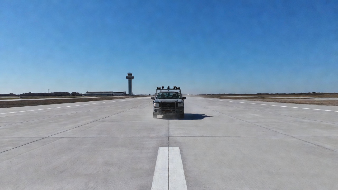
The inertial profiler is the modern replacement for the profilograph, offering significant advantages in speed, accuracy, and safety. First developed by Spangler and Kelley in the 1970s, inertial profilers use a non-contact measurement system that does not require physical contact with the pavement surface. The fundamental components of an inertial profiler are:
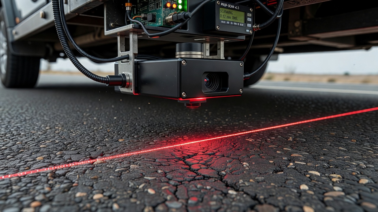
Height Sensor: A laser, infrared, or ultrasonic sensor mounted on the vehicle at a fixed location measures the distance from the sensor to the pavement surface. Laser sensors are the most common type used today, with measurement rates of 16 kHz to 64 kHz and accuracy of ±0.1 mm or better. Single-spot (point) lasers and line lasers are both used; line lasers are preferred on textured concrete surfaces as they better represent the contact area of a tire footprint.
Accelerometer: A high-precision accelerometer mounted integrally with the height sensor measures the vertical acceleration of the vehicle body as it traverses the pavement. The acceleration data is mathematically double-integrated to determine the vertical displacement of the sensor itself. This compensates for the vehicle’s bounce and pitch motions, which would otherwise corrupt the profile measurement.
Distance Measuring System: A distance measuring instrument (DMI), typically using a wheel-mounted encoder or a non-contact sensor, records the longitudinal distance traveled. The DMI triggers data collection at specified intervals (typically 1 inch or less for Class 1 profilers).
Computer and Software: A data acquisition system records the sensor data and performs real-time computation of the pavement profile. The profile elevation is calculated as: Profile Elevation = ∫∫(Acceleration dt²) − Height Sensor Reading. Modern systems also provide immediate computation of IRI, display of profile traces, and reporting of smoothness statistics.
Inertial profilers operate at posted highway speeds (50 to 70 mph) and collect data in both wheelpaths simultaneously. A single operator can perform testing without lane closures (traffic control is generally not required) and can measure 50 to 100 miles of pavement per hour. The data is repeatable, reproducible, and traceable to international standards. ASTM E950 defines three classes of inertial profilers based on sampling interval and accuracy, with Class 1 being the most precise (sampling interval ≤ 1 inch, elevation accuracy ± 0.01 inch).
Two types of inertial profilers are used for construction acceptance testing: high-speed inertial profilers (van-based systems for network-level data collection) and lightweight inertial profilers (utility vehicle-based systems for new construction testing). Lightweight profilers are essential for testing new concrete pavements because they can operate on pavement that has not yet achieved sufficient strength to support a full-size van. Many lightweight profilers can test concrete pavement within hours of placement.

A walking profiler — also known as a walking speed profiler, Dipstick®, or inclinometer profiler — is a low-speed, high-accuracy reference device used to calibrate inertial profilers and to measure pavement profiles in confined areas where full-size profilographs or inertial profilers cannot operate. Walking profilers are classified into two types: inclinometer-based and external-reference-based.
Inclinometer walking profilers measure the pavement profile by recording the slope of the instrument at each measurement interval. The operator walks the device along the pavement, stopping at each measurement point (typically every 6 to 12 inches) to record the slope reading. A computer integrates the slope data to construct the longitudinal elevation profile. These devices are highly accurate, with elevation precision of ±0.001 inches, but very slow — a typical walking profiler covers only 0.5 to 1 mile per hour. They are used primarily as reference standards for certification of inertial profilers and for evaluating short sections where high accuracy is required.
External-reference walking profilers use a non-contact sensor (typically a laser) mounted on a mobile frame that maintains a fixed external reference, such as a stretched wire or a precision level. These devices measure the vertical distance from the external reference to the pavement surface at regular intervals. They are the fastest of the walking profilers and can measure true profile with respect to mean sea level.
Walking profilers play a critical role in the certification and calibration process for inertial profilers. AASHTO R56 (Certification of Inertial Profiling Systems) and AASHTO R57 (Operating Inertial Profiling Systems) specify that inertial profilers must demonstrate their accuracy by comparing their measurements against a reference profile obtained using a walking profiler or rod and level survey. The walking profiler data serves as the ground truth against which the high-speed device’s performance is validated.
Smoothness specifications form the contractual basis for quality control and acceptance of new pavement construction. These specifications define the allowable limits for Profile Index (when using profilographs) or IRI (when using inertial profilers), the sampling and testing protocols, the location and number of test tracks, the identification and correction of localized roughness, and the incentive/disincentive payment adjustments based on achieved smoothness levels.
Highway Pavements: Based on a 2014 FHWA survey, 39 states (78%) were using IRI for asphalt pavement smoothness specifications and 23 states (46%) for concrete pavements. Typical IRI acceptance limits for new highway pavements range from 52 to 72 in/mi (810 to 1130 mm/km). For agencies still using profilograph-based specifications, typical PI acceptance limits range from 7 to 10 in/mi for 0.2-inch blanking band and 20 to 45 in/mi for zero blanking band. Many agencies use a performance-related specification (PRS) approach that provides full payment for pavements meeting target smoothness, with graduated pay reductions for rougher pavements and bonuses for exceptionally smooth pavements.
Airfield Pavements: The FAA Advisory Circular AC 150/5370-10 (Standards for Specifying Construction of Airports) specifies smoothness requirements for airfield pavements. Item P-501 (Portland Cement Concrete Pavement) requires the use of a 16-foot straightedge for smoothness assessment of new concrete pavement. The criteria specify that the surface deviation shall not exceed 1/4 inch when measured with a 16-foot straightedge placed anywhere on the pavement. For asphalt pavements (P-401), similar straightedge criteria apply. The FAA has developed the Straightedge Smoothness Index (SSI) as an automated alternative that emulates the physical straightedge using profile measurements from certified profilers. The Innovative Pavement Research Foundation (IPRF) report 01-G-002-02-4 provides comprehensive guidance on airfield concrete pavement smoothness, including target SSI values and profiler evaluation criteria. For airport runways, the keel section (center 50 feet of the runway divided equally left and right of centerline) receives particular attention due to its critical role in aircraft operations.
The table below summarizes typical smoothness specification limits:
| Parameter | Highway (Asphalt) | Highway (Concrete) | Airfield (Concrete) |
|---|---|---|---|
| Common Metric | IRI | IRI or PI | Straightedge |
| Typical IRI Limit | 52-66 in/mi | 57-72 in/mi | Not applicable |
| Typical PI Limit (0.2" BB) | 7-10 in/mi | 7-10 in/mi | Not applicable |
| Typical PI Limit (0" BB) | 20-45 in/mi | 20-45 in/mi | Not applicable |
| Straightedge Limit | Not applicable | Not applicable | 1/4 inch in 16 ft |
| Source Standard | AASHTO M328 | AASHTO M328 | FAA AC 150/5370-10 |
Smoothness acceptance testing is the formal process of measuring pavement smoothness against specification requirements to determine whether the constructed pavement is acceptable and to calculate any payment adjustments. The testing protocol varies by agency but generally follows these principles:
Test Timing: For concrete pavements, testing should be performed as soon as the concrete has gained sufficient strength to support the testing equipment without damage — typically 3 to 14 days after placement for profilographs, and within hours for lightweight inertial profilers. For asphalt pavements, testing is performed after the pavement has cooled to ambient temperature and before the project is opened to traffic.
Test Tracks: Specifications typically define specific wheelpaths to be tested. Highway specifications commonly require testing in both the left and right wheelpaths of each lane. Airfield specifications may require testing in multiple tracks across the pavement width, including the keel section. The California profilograph typically tests one wheelpath per pass.
Segment Length: Profile data is analyzed in fixed-length segments. Highway specifications commonly use 0.1-mile (528-foot) segments. Airfield specifications may use 100-meter or station-length segments. The segment length must be long enough to provide a meaningful statistical measure of smoothness but short enough to identify localized areas of poor quality.
Localized Roughness: In addition to the overall smoothness index (PI or IRI), specifications identify localized areas of excessive roughness — called must grinds in profilograph specifications and areas of localized roughness in IRI specifications. These are isolated bumps or dips that exceed a specified threshold regardless of the overall smoothness of the segment. Typical thresholds are 0.3 inches deviation in 25 feet for profilograph specifications and a continuous IRI calculation over a 25-foot moving window for inertial profiler specifications. All localized roughness deviations must be corrected by grinding or other approved methods.
Payment Adjustments: Most smoothness specifications include incentive and disincentive payment provisions. Pavements that exceed the target smoothness receive a bonus payment (typically 2% to 5% of the contract unit price), while pavements that fall below the acceptable threshold receive reduced payment. Pavements that fail to meet the minimum acceptable smoothness may require removal and replacement or substantial corrective work at the contractor’s expense.
The relationship between measured smoothness and perceived ride quality is complex and depends on vehicle characteristics, speed, and human sensitivity to vibration. The quarter-car model used for IRI calculation was designed to match the response characteristics of a typical passenger vehicle, and extensive research has demonstrated strong correlation between IRI values and human perception of ride quality. The generally accepted ride quality thresholds for IRI (measured at 50 mph) are:
| IRI (in/mi) | IRI (m/km) | Ride Quality Rating |
|---|---|---|
| < 60 | < 0.95 | Very Good (new pavement) |
| 60 - 95 | 0.95 - 1.50 | Good |
| 95 - 140 | 1.50 - 2.20 | Fair |
| 140 - 200 | 2.20 - 3.15 | Poor |
| > 200 | > 3.15 | Very Poor |
Profilograph-derived Profile Index (PI) does not have the same direct relationship with ride quality as IRI, primarily because the profilograph’s frequency response characteristics introduce wavelength-dependent bias. A pavement that yields an acceptable PI may still exhibit poor ride quality if the roughness is concentrated in wavelength ranges that the profilograph attenuates. Conversely, a pavement with unacceptable PI may provide acceptable ride quality if the roughness is in wavelength ranges that the profilograph amplifies. This limitation of the profilograph has been a primary driver for the industry transition to inertial profilers and IRI-based specifications.
The Ride Number (RN), developed by the University of Michigan Transportation Research Institute (UMTRI), is an alternative smoothness index that estimates the mean panel rating (user perception) from pavement profile data. RN values range from 0 (impassable) to 5 (perfect ride). RN is calculated using a mathematical model that simulates both the vehicle response and the human perception of vibration. Some agencies, including the Florida Department of Transportation (FDOT), use RN in addition to or instead of IRI for smoothness acceptance.
The relationship between initial pavement smoothness and long-term pavement performance is well established through decades of research, most notably by the FHWA Long-Term Pavement Performance (LTPP) program. Smoother pavements consistently demonstrate:
Extended Service Life: Pavements constructed with better initial smoothness maintain acceptable ride quality for a longer period and require less frequent rehabilitation. Research indicates that pavements in the smoothest quartile of initial smoothness can have a service life 20% to 30% longer than those in the roughest quartile. The mechanism is related to reduced dynamic loading: a smooth pavement generates lower dynamic tire forces, which reduces the stress on the pavement structure and delays the development of structural distress.
Reduced Dynamic Loading: Rough pavements cause vehicle tires to bounce and oscillate, generating dynamic impact forces that can be 1.5 to 2.5 times the static tire load. These amplified forces accelerate pavement deterioration through increased fatigue damage, faster rutting, and more rapid crack propagation. Smooth pavements minimize this dynamic amplification, allowing the pavement to perform as designed.
Lower Life-Cycle Costs: The combination of extended service life, reduced maintenance requirements, and lower user costs (fuel consumption, vehicle maintenance, travel time) makes initially smooth pavements more cost-effective over their full life cycle. A study by the FHWA estimated that improving initial smoothness from the 50th percentile to the 10th percentile could reduce life-cycle costs by 10% to 15% for typical highway pavements.
User Satisfaction and Safety: Smooth pavements provide better tire-road contact, improving braking performance, steering response, and overall vehicle control. They reduce driver fatigue and improve comfort, contributing to safer driving conditions. The economic benefits of reduced fuel consumption (2% to 5% reduction on smooth pavements versus rough pavements) and reduced vehicle maintenance costs are significant at the network level.
For these reasons, investment in smoothness during construction — through proper specification, testing, and quality control — is one of the most cost-effective strategies for achieving long-term pavement performance. The profilograph, despite its limitations, has served as the primary tool for this purpose for over 80 years and continues to be specified by many agencies. The trend toward inertial profilers and IRI-based specifications represents an evolution in measurement technology, not a departure from the fundamental principle that smoothness matters.
The following standards govern profilograph testing and pavement smoothness measurement:
| Standard | Title | Key Provisions |
|---|---|---|
| ASTM E1274 | Standard Test Method for Measuring Pavement Roughness Using a Profilograph | Defines the profilograph, test procedure, and data reduction methods |
| ASTM E950 | Standard Test Method for Measuring the Longitudinal Profile of Traveled Surfaces with an Accelerometer-Established Inertial Reference | Classifies inertial profilers (Class 1-3) based on accuracy |
| ASTM E1926 | Standard Practice for Computing International Roughness Index of Roads from Longitudinal Profile Measurements | Defines the IRI quarter-car algorithm |
| AASHTO R56 | Standard Practice for Certification of Inertial Profiling Systems | Specifies certification procedures for inertial profilers |
| AASHTO R57 | Standard Practice for Operating Inertial Profiling Systems | Specifies operational procedures for inertial profiling |
| California Test Method 526 | Method of Test for Determining Profile Index of Pavement Surfaces | Defines profilograph operation, trace reduction, and PI calculation |
| FAA AC 150/5370-10 | Standards for Specifying Construction of Airports | Specifies straightedge and smoothness requirements for airfield pavements |
| ASTM E867 | Standard Terminology Relating to Vehicle-Pavement Systems | Defines standard pavement roughness and profile terminology |
TarmacView provides comprehensive pavement inspection services including profilograph testing, inertial profiling, and IRI analysis for airport runways, highways, and airfield pavements. Contact our team for expert smoothness assessment and quality control.
A vehicle-mounted inertial profiler uses laser height sensors and accelerometers to measure longitudinal pavement profile at highway speeds, computing IRI and r...
Comprehensive glossary of profile (longitudinal) and vertical cross-section surveying in civil engineering, covering methods, applications, terminology, and sta...
The International Roughness Index (IRI) is a standardized longitudinal profile-based measure of pavement roughness, expressed in m/km or in/mi. Developed by the...