Smoke Test
A smoke test is a quick, end-to-end verification that a software pipeline executes without crashing on representative data, producing expected outputs. TarmacVi...
32 min read
testing
technology
+4
The defect head smoke test validates that TarmacView’s structural defect detection pipeline — DINOv3 backbone + 5-label MLP head for crack/spalling/efflorescence/exposed_rebar/corrosion — produces expected outputs on test data. Covers test assertions (checkpoint exists; AP metrics; tile/frame defect columns in analyze output) and what smoke tests verify vs full evaluation.
Defect head smoke testing is an automated verification procedure that validates the structural integrity and basic functionality of a defect detection machine learning pipeline. It confirms that the pipeline — from input image preprocessing through the DINOv3 vision transformer backbone to the 5-label Multi-Layer Perceptron (MLP) classification head — produces expected outputs on synthetic or small static test data without crashing, producing numerical errors, or generating structurally invalid predictions. The smoke test is distinct from a full evaluation: it verifies that the pipeline is correctly wired and operational, not that it generalizes to unseen data with high accuracy.
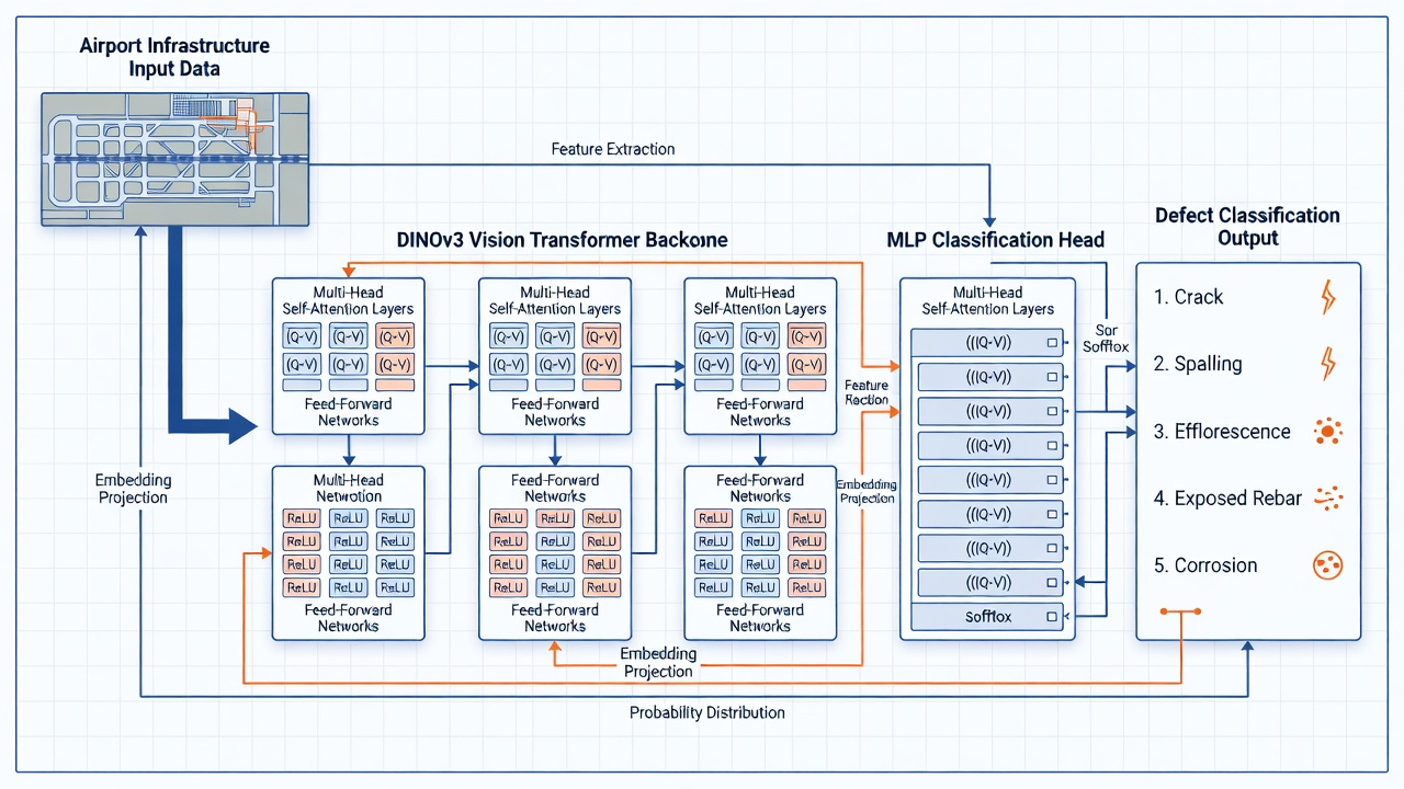
The defect head is the final component of TarmacView’s structural defect detection pipeline, responsible for mapping the rich feature representations extracted by the backbone network to discrete defect class predictions. Understanding the architecture of both the backbone and the head is essential for designing effective smoke tests that validate each component’s integrity.
The DINOv3 (self-DIstillation with NO labels, version 3) vision transformer, developed by Meta AI and released in 2023, serves as the feature extraction backbone. DINOv3 was trained using a self-supervised learning paradigm on a curated dataset of 142 million unlabeled images (LVD-142M), learning general-purpose visual representations without requiring any human annotations. This approach produces features that transfer effectively to downstream tasks including defect classification, segmentation, and detection — often outperforming supervised pretraining on ImageNet-1K.
DINOv3 is available in multiple model variants with different computational profiles:
| Variant | Parameters | Embedding Dim | Patch Size | Layers | Heads |
|---|---|---|---|---|---|
| ViT-S/14 | 22 million | 384 | 14×14 | 12 | 6 |
| ViT-B/14 | 86 million | 768 | 14×14 | 12 | 12 |
| ViT-L/14 | 300 million | 1024 | 14×14 | 24 | 16 |
| ViT-g/14 | 1.1 billion | 1536 | 14×14 | 40 | 24 |
For TarmacView’s defect detection pipeline, the ViT-B/14 variant is the standard configuration. With 86 million parameters and a 768-dimensional embedding space, it balances representational capacity with computational efficiency suitable for processing large volumes of runway inspection imagery. The 14×14 patch size means that a 224×224 pixel input image is divided into 16×16 = 256 non-overlapping patches, each projected into the 768-dimensional embedding space through a learned linear projection.
The DINOv3 training methodology combines several key techniques. Self-distillation with teacher-student architecture ensures that the student network learns to match the teacher’s representations, with the teacher being an exponential moving average of the student. iBOT (image BERT pre-training with Online Tokenizer) applies masked image modeling, where random patches are masked and the model must predict the masked patch representations. Sinkhorn-Knopp centering from the SwAV method prevents representation collapse by enforcing uniform distribution across batch samples. KoLeo regularizer encourages diversity in the learned features by penalizing feature similarity between nearby samples.
For the defect detection use case, DINOv3 is loaded with pretrained weights and typically frozen during defect head training. The frozen backbone extracts general visual features — edges, textures, gradients, surface patterns — that are highly relevant for distinguishing between intact pavement and the five defect classes. Freezing the backbone reduces the number of trainable parameters from 86 million to approximately 1-3 million (depending on MLP head depth), dramatically reducing training time, GPU memory requirements, and the risk of catastrophic forgetting on small domain-specific datasets.
The MLP (Multi-Layer Perceptron) defect head is a small feedforward neural network that takes the frozen DINOv3 embeddings as input and produces a 5-dimensional probability distribution over the five defect classes: crack, spalling, efflorescence, exposed rebar, and corrosion.
The standard architecture consists of:
Input layer: Accepts the DINOv3 embedding — either the [CLS] token (a 768-dimensional vector representing global image content) or a pooled representation of all patch tokens. The [CLS] token approach is standard because DINOv3 is specifically trained to produce rich information in the [CLS] token during self-distillation.
Hidden layers: Typically 1-2 fully connected layers with ReLU or GELU activation functions. A single hidden layer configuration might be 768 → 256 → 5, while a deeper configuration might be 768 → 512 → 128 → 5. Each hidden layer is followed by batch normalization or layer normalization to stabilize training and reduce internal covariate shift. Dropout (rate 0.2-0.5) is applied between hidden layers during training as a regularizer to prevent overfitting, given that infrastructure defect datasets are typically small (500-5000 images).
Output layer: A linear projection to 5 units corresponding to the five defect classes, followed by a softmax activation that converts logits to a probability distribution over the classes. The softmax function ensures that the output vector sums to 1.0, with each element representing the predicted probability that the input image belongs to that defect class.
Training procedure: The MLP head is trained via supervised fine-tuning while the DINOv3 backbone remains frozen. The loss function is categorical cross-entropy, comparing the predicted probability distribution against the one-hot encoded ground truth labels. Training typically uses the AdamW optimizer with a learning rate of 1e-3 to 1e-4, batch size of 32-128, and early stopping based on validation loss. Data augmentation (random rotation, horizontal flip, color jitter, random crop) is applied during training to improve generalization.
For inference, the DINOv3 backbone processes each input image into patch and [CLS] token embeddings in a single forward pass. The [CLS] embedding is extracted and passed through the MLP head. The output softmax probabilities are thresholded (typically at 0.5 or optimized via ROC analysis) to produce a binary prediction for each defect class. Because the five defect classes are not mutually exclusive — a single pavement area can exhibit both cracking and spalling simultaneously — the thresholded predictions for each class are independent, and the output is properly interpreted as multi-label rather than single-class prediction.
In the TarmacView analysis pipeline, the defect head operates at two granularity levels.
Tile-level analysis: The runway surface is divided into a grid of image tiles (typically 224×224 or 512×512 pixels at the inspection resolution of 0.5-2.0 mm/pixel). Each tile is processed independently through the DINOv3 backbone and MLP defect head, producing a 5-element probability vector per tile. Tile-level predictions are stored as per-tile columns in the analysis output: tile_crack_conf, tile_spalling_conf, tile_efflorescence_conf, tile_exposed_rebar_conf, tile_corrosion_conf.
Frame-level aggregation: Individual tile predictions within a camera frame or runway section are aggregated to produce frame-level defect assessments. Aggregation methods include: max pooling (the maximum confidence across all tiles in the frame), mean pooling (average confidence), top-k voting (the proportion of tiles exceeding a threshold), and spatial density (the count of defect tiles per unit area). Frame-level columns in the output include frame_crack_flag, frame_spalling_flag, frame_defect_count, and frame_max_defect_conf.
The analysis output schema is a critical component that smoke tests must validate. If the tile-level confidence columns or frame-level aggregation columns are missing, renamed, or contain invalid values (NaN, inf, negative probabilities), downstream Pavement Condition Index (PCI) calculations and reporting pipelines will fail.
Smoke test assertions are the specific, automated checks that verify the defect head pipeline is functioning correctly. Each assertion targets a specific failure mode and produces a clear pass/fail result that can be integrated into CI/CD pipeline gating.
The first category of smoke test assertions verifies that the defect head checkpoint — the saved model weights file — is valid and loadable. The assertions include:
Checkpoint file existence: The test asserts that the checkpoint file exists at the specified path. This catches issues where a training run failed, the checkpoint was not uploaded to the model registry, or the file path was incorrectly configured in the deployment environment. The assertion is: assert os.path.exists(checkpoint_path), f"Checkpoint not found at {checkpoint_path}".
File size and checksum validation: The test verifies that the checkpoint file has a non-zero file size and optionally validates its MD5 or SHA256 checksum against a stored baseline. A zero-byte file or corrupted download will be caught here. The assertion is: assert os.path.getsize(checkpoint_path) > 0 and optionally assert sha256(file) == expected_sha256.
Torch loadability: The test loads the checkpoint using torch.load() and asserts that the operation completes without throwing an exception. This catches corrupted files, version incompatibilities (e.g., a checkpoint saved with PyTorch 2.0 attempting to load with PyTorch 1.8), and missing dependencies. The assertion wraps the load call in a try/except block and fails on any exception.
State dictionary structure: After loading, the test asserts that the checkpoint contains the expected state dictionary keys. For the DINOv3 backbone, expected keys include backbone.cls_token, backbone.patch_embed.proj.weight, and transformer block parameters. For the MLP head, expected keys include head.0.weight, head.0.bias, head.2.weight, head.2.bias (for a 2-layer MLP). The test also verifies that all expected keys are present and that no unexpected keys exist, which could indicate a model architecture mismatch.
The second category verifies that a forward pass through the combined backbone and head produces valid outputs.
Tensor shape validation: The test creates a synthetic input tensor of the expected shape (typically [batch_size, 3, height, width] with batch_size=1-4, height=width=224 for ViT-B/14), passes it through the model, and asserts that the output tensor shape is [batch_size, 5] — exactly 5 logits corresponding to the 5 defect classes. The assertion is: assert output.shape == (batch_size, 5), f"Expected shape (batch_size, 5), got {output.shape}".
Numerical stability validation: The test asserts that no output value is NaN (Not a Number), infinity, or negative infinity. NaN values can arise from numerical instability in the transformer backbone (e.g., attention logit overflow), division by zero in normalization layers, or corrupted weights. The assertion is: assert not torch.isnan(output).any(), "Output contains NaN values" and assert not torch.isinf(output).any(), "Output contains inf values".
Softmax probability validation: The test applies softmax to the raw logits and asserts that the resulting probabilities sum to 1.0 for each sample in the batch (within floating-point tolerance, typically 1e-5). This confirms that the output layer is correctly configured and that no post-processing step is corrupting the probability distribution. The assertion is: assert torch.allclose(probs.sum(dim=1), torch.ones(batch_size), atol=1e-5).
The third category verifies that the model produces reasonable prediction distributions rather than degenerate outputs.
Non-uniform distribution check: The test asserts that the predicted probabilities are not uniform across all classes (which would indicate a model that has not learned any discriminative features). The entropy of the predicted distribution is computed and compared against a minimum threshold. A completely uniform distribution has maximum entropy (log(5) ≈ 1.61 nats for 5 classes), while a confident prediction has low entropy. The assertion is: assert entropy < 1.5, "Predictions are near-uniform, model may not be trained".
Class coverage check: The test runs inference on a small set of diverse input images and asserts that each of the 5 defect classes is the highest-confidence prediction for at least one input. This verifies that no class is systematically suppressed — for example, a model that never predicts “efflorescence” would indicate a training data imbalance or head configuration issue. The assertion is: assert set(predicted_classes) == set(range(5)), f"Classes {missing} never predicted".
Background class handling: If the model includes an implicit background or “no defect” class, the smoke test verifies that an image of intact pavement — free of any defect — produces a background prediction with confidence above a threshold (typically 0.8). This confirms that the model can correctly reject negative examples, which is critical for avoiding false positive alarms in production inspections.
Checkpoint validation is a foundational smoke test component that confirms the model artifact — the saved neural network weights — is intact, loadable, and structurally consistent with the expected architecture. In production ML systems, checkpoint corruption or version mismatch is one of the most common failure modes, and catching it early in CI/CD prevents cascading failures downstream.
TarmacView defect head checkpoints are stored in the model registry — a centralized artifact store with versioning, metadata, and lineage tracking (MLflow Model Registry or DVC). Each checkpoint is identified by a unique combination of model name, version number, and run ID. The checkpoint file itself is a serialized PyTorch state dictionary (typically model.pt or checkpoint.pt) containing the learned parameters of both the DINOv3 backbone (if fine-tuned) and the MLP head.
The smoke test first resolves the checkpoint path from the model registry, handling the following cases:
defect-head:v3), and the test loads that exact version.The DINOv3 backbone is a large model with 86 million parameters for the ViT-B/14 variant. The smoke test verifies that the loaded backbone matches the expected architecture by checking:
Weight tensor shapes: Each parameter tensor in the loaded state dictionary is verified against the expected shape. For example, the backbone.patch_embed.proj.weight tensor should have shape (768, 3, 14, 14) for a ViT-B/14 with 3 input channels, 768 output channels, and a 14×14 patch kernel. A shape mismatch would indicate that the checkpoint was trained with a different configuration (different patch size, different embedding dimension, different input channels).
Numerical range sanity: The test verifies that weight values fall within expected numerical ranges. Transformer attention weights should have values distributed roughly as N(0, σ²) with σ depending on the initialization scheme. Extreme values (|w| > 10) across all layers would indicate training divergence or checkpoint corruption. The check computes the mean and standard deviation of each parameter tensor and flags outliers.
Output embedding consistency: The test runs a fixed synthetic input through the backbone and compares the output embedding distribution against a stored baseline. The baseline is generated during the first successful smoke test run and stored as a reference. The assertion checks that the mean and variance of the embedding do not drift beyond a tolerance (typically ±5%). This catches silent model degradation that does not produce NaN or inf values but still produces anomalous embeddings.
The MLP head is smaller than the backbone but equally critical. The smoke test verifies:
Layer count: The head should have exactly the expected number of layers. For a 2-layer MLP with hidden dimension 256, the expected keys include head.0.weight (768×256), head.0.bias (256), head.2.weight (256×5), head.2.bias (5). The layer numbering accounts for the activation function (layer 1) between the linear layers.
Output dimension: The final linear layer’s output dimension must be exactly 5, corresponding to the 5 defect classes. This is verified by checking head.2.weight.shape[0] == 5.
Weight initialization consistency: The test checks that weights are not frozen at initialization values (all zeros or all ones). A head with all-zero weights would produce uniform logits regardless of input, indicating a training failure. The check verifies that head.2.weight.std() > 0.001.
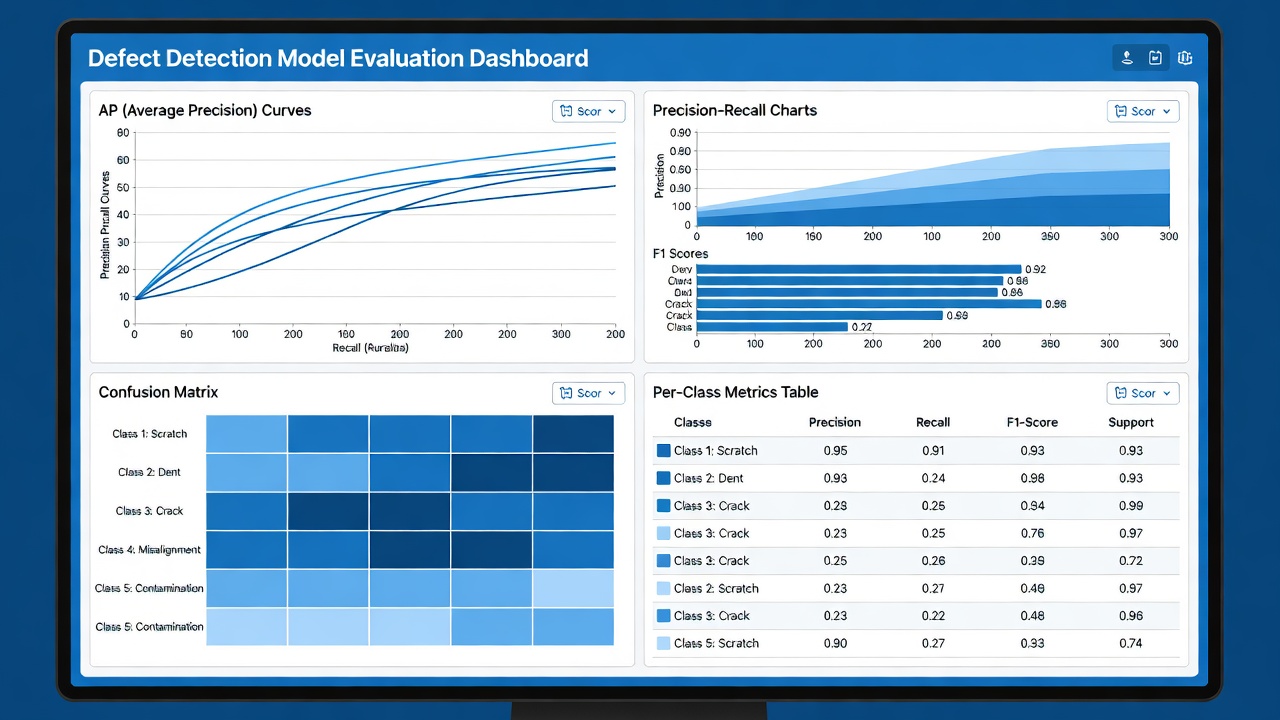
While the smoke test is primarily about pipeline integrity rather than model quality, including lightweight metric computation in the smoke test provides an early warning of significant model regression. The smoke test computes efficacy metrics on synthetic or small static test data, comparing them against baselines stored from previous validated runs.
Average Precision (AP) is the area under the precision-recall curve, computed across confidence thresholds from 0 to 1. The smoke test computes AP for each of the 5 defect classes using COCO-style evaluation:
The smoke test AP assertions include:
AP@0.50 (PASCAL VOC metric): AP at IoU threshold 0.50. The assertion is that AP@0.50 for each class exceeds a minimum threshold. For synthetic test data with known, clean defect patterns, a typical threshold is AP@0.50 > 0.85 for all 5 classes. If the model achieves AP@0.50 below this threshold on trivial synthetic data, it indicates severe regression.
AP@0.50 :0.95 (COCO primary metric): The average of AP values computed at IoU thresholds 0.50, 0.55, …, 0.95. The assertion threshold is lower — typically AP@0.50 :0.95 > 0.50 — because the strict IoU thresholds are more challenging even on synthetic data.
Per-class AP consistency: The variance of AP across the 5 classes is checked. A standard deviation exceeding 0.15 would indicate that one class has regressed significantly relative to others, suggesting a problem specific to that defect type (e.g., insufficient training examples for efflorescence).
The synthetic test dataset is carefully constructed to ensure metric stability. Each synthetic image contains exactly one defect type overlaid on a pavement-like background texture. Defects are generated using procedural techniques: cracks as thin, branched black lines with Gaussian blur for realism; spalls as irregular circular/oval regions with edge roughness; efflorescence as white, amorphous patches with varying opacity; exposed rebar as periodic dark circular patterns; corrosion as rust-colored irregular blobs. The synthetic dataset is versioned and checked into the repository to ensure deterministic, reproducible smoke test results.
F1-score is the harmonic mean of precision and recall, providing a single balanced measure of model performance. The smoke test computes F1 at a fixed confidence threshold (typically 0.5) for each defect class.
The F1 assertions include:
Minimum F1 per class: Each class must achieve F1 > 0.80 on the synthetic test set. The multi-label nature of the defect prediction task means that F1 is computed independently per class.
Macro-averaged F1: The unweighted average of F1 across all 5 classes is computed. The assertion threshold is macro-F1 > 0.85. The macro-average treats all classes equally, so regression on a rare class (e.g., exposed rebar) is immediately visible.
Precision-recall balance: The ratio of precision to recall is checked for each class. A ratio above 1.5 or below 0.67 indicates imbalance — the model is either too conservative (high precision, low recall, missing many defects) or too aggressive (high recall, low precision, generating many false positives). The assertion flags any class where the ratio is outside [0.67, 1.5].
| Metric | Synthetic Test Threshold | Purpose |
|---|---|---|
| AP@0.50 | > 0.85 | Basic detection capability per class |
| AP@0.50 :0.95 | > 0.50 | Comprehensive detection quality |
| Per-class AP std | < 0.15 | Class balance check |
| F1 per class | > 0.80 | Balanced precision-recall per class |
| Macro-averaged F1 | > 0.85 | Overall model quality |
| Precision/Recall ratio | [0.67, 1.5] | Precision-recall balance per class |
The smoke test stores metric baselines from the last validated run and compares current metrics against these baselines. A significant drop (>5% relative decrease) in any metric triggers a smoke test failure, even if the absolute metric value is above the minimum threshold. This catches gradual degradation — models that pass absolute thresholds but are consistently declining in performance across successive training runs or data updates.
Metric histories are logged to a time-series database (MLflow, Weights & Biases, or a simple CSV file in the repository). The smoke test reads the last 10 validated metric values and fits a linear trend. If the slope is negative and statistically significant (p < 0.05), the test outputs a warning but does not fail — threshold-only failure is used for CI/CD gating to avoid noisy pipeline breaks from minor metric fluctuations.
A critical smoke test validates that the analysis output — the structured data produced by running the defect head on inspection imagery — contains all expected columns with correct data types and valid values. This bridges the gap between model inference and downstream Pavement Condition Index (PCI) computation, reporting, and GIS integration.
The TarmacView analysis output is a tabular format (Parquet, CSV, or database table) with columns organized into tiers:
Tile-level defect confidence columns — one float column per defect class, representing the MLP head’s softmax confidence that the tile contains that defect:
| Column Name | Data Type | Valid Range | Description |
|---|---|---|---|
tile_crack_conf | Float32 | [0.0, 1.0] | Probability of crack presence |
tile_spalling_conf | Float32 | [0.0, 1.0] | Probability of spalling presence |
tile_efflorescence_conf | Float32 | [0.0, 1.0] | Probability of efflorescence presence |
tile_exposed_rebar_conf | Float32 | [0.0, 1.0] | Probability of exposed rebar presence |
tile_corrosion_conf | Float32 | [0.0, 1.0] | Probability of corrosion presence |
Frame-level aggregation columns — summarizing defect presence across all tiles in a camera frame or runway section:
| Column Name | Data Type | Valid Range | Description |
|---|---|---|---|
frame_defect_count | Int32 | [0, max_tiles] | Number of tiles with any defect above threshold |
frame_max_defect_conf | Float32 | [0.0, 1.0] | Maximum confidence across all defects and tiles |
frame_crack_flag | Boolean | {0, 1} | Any tile has crack_conf > threshold |
frame_spalling_flag | Boolean | {0, 1} | Any tile has spalling_conf > threshold |
frame_efflorescence_flag | Boolean | {0, 1} | Any tile has efflorescence_conf > threshold |
frame_exposed_rebar_flag | Boolean | {0, 1} | Any tile has exposed_rebar_conf > threshold |
frame_corrosion_flag | Boolean | {0, 1} | Any tile has corrosion_conf > threshold |
Metadata columns — identifying the spatial and temporal context of each analysis record:
| Column Name | Data Type | Description |
|---|---|---|
image_id | String | Unique identifier for the source image |
tile_x | Int32 | Tile column index in the runway grid |
tile_y | Int32 | Tile row index in the runway grid |
frame_timestamp | DateTime | Capture time of the source frame |
gps_lat | Float64 | GPS latitude of the tile center |
gps_lon | Float64 | GPS longitude of the tile center |
The smoke test loads the analysis output and asserts that each expected column exists using simple column-name matching:
expected_tile_cols = ["tile_crack_conf", "tile_spalling_conf",
                      "tile_efflorescence_conf", "tile_exposed_rebar_conf",
                      "tile_corrosion_conf"]
expected_frame_cols = ["frame_defect_count", "frame_max_defect_conf",
                       "frame_crack_flag", "frame_spalling_flag",
                       "frame_efflorescence_flag", "frame_exposed_rebar_flag",
                       "frame_corrosion_flag"]
expected_meta_cols = ["image_id", "tile_x", "tile_y",
                      "frame_timestamp", "gps_lat", "gps_lon"]

actual_cols = set(df.columns)
assert expected_cols.issubset(actual_cols), f"Missing columns: {expected_cols - actual_cols}"
For each defect confidence column, the smoke test asserts:
Float type: The column data type is float32 or float64. Unexpected types (int, string, object) indicate a serialization or pipeline error. The assertion uses assert df[col].dtype in [np.float32, np.float64].
Value range: All values are in [0.0, 1.0]. Values outside this range indicate a softmax or normalization failure. The assertion uses assert df[col].between(0.0, 1.0).all().
Missing value check: No values are NaN or None. NaN values in confidence columns indicate that the inference pipeline produced no output for some tiles — a serious failure. The assertion uses assert df[col].notna().all().
The frame-level columns should be consistent with the tile-level data from which they are derived. The smoke test validates:
frame_defect_count equals count of tiles where max confidence exceeds threshold: For each frame group, the test recomputes the defect count from tile-level data and asserts it matches the stored frame value. This catches aggregation logic errors in the pipeline.
frame_max_defect_conf equals max of all tile confidence values: The test recomputes the maximum from tile-level data and asserts match.
frame_flag is consistent with tile_conf: For each frame, the flag should be 1 if any tile has the corresponding confidence above threshold, and 0 otherwise. The test verifies this for all 5 defect types.
These consistency checks operate on the principle that the frame-level columns should be deterministically derivable from the tile-level columns. If the aggregation logic is correct, the checks should always pass. A failure indicates a bug in the analysis pipeline post-processing step, not in the model itself.
The smoke test compares the expected column set against the actual column set and generates warnings for:
tile_moisture_conf), the test warns but does not fail, as this may indicate a pipeline enhancement that requires downstream integration updates.tile_crack_conf → tile_cracking_conf), the test fails, preventing silent downstream breakage when reporting dashboards, APIs, or databases reference the old column names.The gating logic determines whether the defect head passes or fails the smoke test as a whole, based on a weighted combination of individual assertion results. Gating is the mechanism that prevents a failing model from being deployed to production.
Not all smoke test assertions are equally critical. The gating system assigns each assertion to a severity tier:
| Tier | Weight | Effect on Gate | Examples |
|---|---|---|---|
| Fatal | 1.0 | Gates immediately | Checkpoint load failure, NaN in outputs |
| Critical | 0.8 | Gates if >1 failure | Missing columns, output shape mismatch |
| Warning | 0.4 | Gates if >3 failures | Per-class AP below threshold |
| Info | 0.0 | Logs only, no gate | Metric trend warnings, column deprecation notices |
Fatal assertions are those where no valid pipeline execution is possible — checkpoint is corrupted, model cannot load, or inference produces invalid numerical values. A single fatal failure gates the deployment.
Critical assertions indicate that the pipeline produces structurally valid but potentially incorrect results — missing columns would cause downstream reporting failures, output shape mismatch indicates a model architecture mismatch with the serving infrastructure.
Warning assertions indicate that the model metrics are below nominal thresholds but the pipeline is structurally sound. These are aggregated: if more than 3 warnings fire in a single run, the gate activates.
Info assertions are purely observational — they log metric drift trends, column deprecation notices, and performance comparisons against previous runs — but never gate deployment.
The overall smoke test result is computed as:
gate_score = max(fatal_failures,
                  critical_failures > 1 ? 1.0 : 0.0,
                  warning_failures > 3 ? 1.0 : 0.0)
If gate_score >= 1.0, the smoke test fails and deployment is blocked. If gate_score < 1.0, the smoke test passes, and the pipeline proceeds to full evaluation or deployment.
The composite pass/fail message summarizes the result:
SMOKE TEST: FAIL
  - Fatal: 1 [checkpoint_load_failure]
  - Critical: 0
  - Warning: 2 [class_crack_ap_below_threshold, class_efflorescence_f1_below_threshold]
  - Info: 1 [metric_class_crack_ap dropped 3.2% since last run]
The smoke test gate integrates with the deployment pipeline through:
Post-commit hook: The smoke test runs on every pull request commit. If the gate fails, the CI/CD system blocks the merge (GitHub branch protection rule, GitLab merge request pipeline failure).
Pre-deployment gate: Before a model is promoted from staging to production, the smoke test runs again on the exact deployment candidate artifact. This catches issues that may not have been present during development — for example, a development environment with different CUDA version than the production serving environment.
Rollback trigger: If the smoke test passes deployment but a subsequent production incident is traced to the defect head, the smoke test gating logic is audited. If a warning-level assertion should have been a critical assertion, the gating configuration is updated to prevent recurrence.
Domain applicability tests extend the basic smoke test to verify that the defect head performs correctly across the specific operational conditions that TarmacView encounters in airfield pavement and infrastructure inspection. These tests ensure that the pipeline is not only functional but fit for purpose in the target domain.
The defect head must perform consistently across different pavement types encountered on airport surfaces:
Asphalt (flexible) pavements: Runways, taxiways, and aprons constructed with hot mix asphalt (HMA). Defects on asphalt include fatigue cracking (alligator pattern), longitudinal cracking, transverse cracking, rutting, and raveling. The smoke test includes synthetic images with asphalt-like textures (dark gray, aggregate visible, varying surface roughness) and verifies that crack and spalling detection maintain nominal confidence levels.
Concrete (rigid) pavements: Runways and aprons constructed with Portland cement concrete (PCC). Defects include joint spalling, corner breaks, linear cracking, efflorescence (white calcium deposits at joints), exposed rebar (at spalled areas), and corrosion staining. The smoke test verifies that the model correctly identifies efflorescence and exposed rebar — defects that are far more prevalent on concrete than asphalt surfaces.
Composite pavements: Asphalt overlays on existing concrete. Defects include reflective cracking (asphalt cracks following underlying concrete joint pattern) and delamination. The test verifies that the model can detect cracks on composite surfaces without confusion from the underlying joint pattern.
Porous friction courses (PFC): High-permeability asphalt used on runways for improved drainage and friction. PFC has a distinctive open-graded texture that appears visually different from dense-graded HMA. The test verifies that the model does not produce elevated false positive rates on PFC surfaces, where the rough texture might be confused with cracking or spalling.
ICAO Annex 14 and FAA AC 150/5320-5D specify that runway surface condition assessments must be valid under operational conditions. The domain applicability smoke test verifies that the defect head maintains performance across:
Direct sunlight: High contrast, strong shadows. The test verifies that confidence values are not systematically lower in high-contrast conditions due to shadow-induced false positives.
Overcast/diffuse light: Low contrast, no shadows. The test verifies that fine cracks (narrow, low contrast against pavement) are still detectable at reduced confidence levels.
Wet pavement: Water in cracks increases crack visibility but introduces specular reflections. The test verifies that wet surface tiles do not produce elevated false positives due to specular highlights being confused with efflorescence (both appear as bright regions).
Dawn/dusk: Low light levels, long shadows. The test verifies that the model produces outputs within expected confidence ranges even at reduced illumination levels.
The smoke test simulates these conditions by applying controlled photometric transforms to the synthetic test images: brightness scaling for lighting simulation, Gaussian blur for haze/fog simulation, and saturation adjustment for wet surface simulation.
Inspection imagery varies in ground sampling distance (GSD) depending on the capture platform:
| Platform | Typical Altitude | GSD (mm/pixel) | Tile Coverage |
|---|---|---|---|
| UAV (high resolution) | 15-20 m | 0.5-1.0 | 0.1-0.5 m² |
| UAV (standard) | 30-50 m | 1.0-2.0 | 0.5-2.0 m² |
| Vehicle-mounted | 2-3 m | 0.3-0.8 | 0.05-0.2 m² |
| Handheld | 1-1.5 m | 0.2-0.5 | 0.02-0.08 m² |
The smoke test verifies that the defect head produces consistent outputs across a range of input resolutions. Synthetic test images are generated at multiple scales (0.5×, 1.0×, 2.0× the nominal GSD) and passed through the model. The test asserts that the predicted class distribution does not shift by more than 10% between resolutions, ensuring the model is approximately scale-invariant within the operational range.
ASTM D5340 defines three severity levels (Low, Medium, High) for each defect type. The smoke test verifies that the defect head’s confidence scores correlate with defect severity:
Low severity: Hairline cracks (<1mm width), small spalls (<150mm length), light efflorescence, minimal corrosion staining. The test asserts that these produce confidence scores above the detection threshold (>0.5) but not at maximal confidence (<0.8).
Medium severity: Cracks (1-3mm width), spalls (150-600mm length), moderate efflorescence deposits, visible exposed rebar with light corrosion. The test asserts that confidence scores are high (>0.7).
High severity: Wide cracks (>3mm width), large spalls (>600mm length), heavy efflorescence with surface disruption, exposed rebar with heavy corrosion and section loss. The test asserts that confidence scores are very high (>0.9).
Severity correlation verification is a warning-level assertion in the gating system — the model may still function correctly even if severity correlation is imperfect, but the test flags it as an area for model improvement.
Understanding the distinction between smoke testing and full evaluation is critical for designing an effective ML quality assurance strategy. The two approaches serve fundamentally different purposes and operate at different points in the development and deployment lifecycle.
| Dimension | Smoke Test | Full Evaluation |
|---|---|---|
| Goal | Verify pipeline integrity | Measure model quality |
| Question answered | “Does the pipeline run correctly?” | “Is the model accurate enough?” |
| Data | Synthetic / small static set (10-100 images) | Large held-out validation set (500-5000+ images) |
| Duration | Seconds to minutes | Minutes to hours |
| Compute | CPU or minimal GPU | Full GPU (often multi-GPU) |
| Frequency | Every commit / PR | Nightly, weekly, or per-release |
| Metric thresholds | Generous (AP > 0.50) | Stringent (AP > 0.75) |
| Coverage | Structural integrity only | Statistical generalization |
| Failure action | Block merge/deployment | Flag for review |
The smoke test is designed to catch pipeline errors — the class of bugs that cause the entire system to fail or produce meaningless outputs. These include checkpoint corruption, version incompatibility, preprocessing pipeline breaks, missing columns, NaN outputs, and shape mismatches. Industry data from ML engineering teams shows that pipeline errors account for 60-70% of failed training runs and 40% of deployment rollbacks. Smoke tests catch these errors in seconds, before expensive full evaluation runs are initiated.
The full evaluation is designed to measure model quality — the statistical accuracy, precision, recall, and generalization of the model’s predictions. It uses large, diverse, representative validation datasets, computes rigorous metrics (AP@0.50 :0.95, class-wise F1, confusion matrices, precision-recall curves at multiple thresholds), and compares results against both absolute thresholds and relative baselines from previous model versions. Full evaluation runs are computationally expensive and time-consuming, making them unsuitable for per-commit execution.
Smoke test data is synthetically generated to be simple, clean, and deterministic. Each synthetic image contains exactly one defect type on a uniform background, with no occlusion, no overlapping defects, and no challenging lighting conditions. This minimizes variability and ensures that any metric fluctuation in the smoke test is attributable to the model, not to data variability.
Full evaluation data is real-world inspection imagery with the following characteristics: diverse pavement types and ages, all operational lighting conditions, varying defect severity levels, overlapping and adjacent defects, real-world occlusions (debris, tire marks, water), and accurate polygon-level ground truth annotations. This data represents the true distribution that the model encounters in production and provides a reliable estimate of deployment performance.
Data leakage prevention is critical for full evaluation but irrelevant for smoke tests — since the smoke test uses synthetic data, there is no risk of leaking real test data into training. The full evaluation dataset is carefully partitioned: training, validation, and test sets are split at the frame or runway level (not the tile level) to prevent spatial autocorrelation leakage, where adjacent tiles from the same runway appear in both training and test sets.
A typical smoke test run for the defect head pipeline:
A typical full evaluation run:
The smoke test is 10-100× faster than the full evaluation, enabling per-commit execution. The full evaluation runs on a slower cadence (per-night, per-release, per-promotion to production).
| Failure Mode | Detected By |
|---|---|
| Corrupted checkpoint file | Smoke test (fatal) |
| NaN/inf in model outputs | Smoke test (fatal) |
| Missing output columns | Smoke test (critical) |
| Wrong output tensor shape | Smoke test (critical) |
| Preprocessing normalization mismatch | Smoke test (fatal) |
| Degenerate predictions (all same class) | Smoke test (warning) |
| 10% AP drop on new data | Full evaluation |
| Overfitting to a specific pavement type | Full evaluation |
| Calibration drift | Full evaluation |
| Label noise in training data | Full evaluation |
The coverage matrix demonstrates that smoke tests and full evaluations are complementary — each catches failure modes that the other misses. A comprehensive ML testing strategy requires both.
Integration of the defect head smoke test into continuous integration (CI) pipelines is essential for catching regressions early and ensuring that every code change is validated before affecting production systems.
The CI pipeline for TarmacView’s defect detection system is organized into sequential stages:
Stage 1 — Code Quality: Linting (flake8, pylint), type checking (mypy), unit tests (pytest for data-loading utilities, preprocessing functions, and metric computation functions). This stage runs on CPU and completes in 1-3 minutes. Failure blocks all downstream stages.
Stage 2 — Data Validation: Schema validation of training and evaluation datasets using Great Expectations or TensorFlow Data Validation. Checks column presence, data types, value ranges, and distribution statistics against expectations defined in the data contract. This stage runs on CPU and completes in 2-5 minutes.
Stage 3 — Defect Head Smoke Test: The full smoke test suite as described in this article. Runs on CPU (or minimal GPU if available) and completes in 15-60 seconds. Failure blocks merge to main.
Stage 4 — Unit Tests for Evaluation: Small-scale metric computation tests that verify AP computation, F1 computation, and confusion matrix generation produce correct outputs on hand-labeled tiny datasets (5-10 images with known ground truth). Runs on CPU, completes in 30 seconds.
Stage 5 — Training (on demand): Triggered only when model weights are expected to change (new training data, architecture changes, hyperparameter tuning). Not automatically triggered on every commit. Runs on GPU and takes 1-8 hours depending on dataset size.
Stage 6 — Full Evaluation (on merge to main): Triggered when code is merged to the main branch. Runs the complete evaluation suite on the held-out validation set, computes all metrics, compares against baselines, and publishes results to the model registry. Runs on GPU and takes 20-40 minutes.
The smoke test is triggered on:
CI artifacts from the smoke test are stored and versioned:
These artifacts are stored in the model registry alongside the model artifact itself, providing a complete audit trail: “This version of the model passed the smoke test with synthetic data v3.2 on CI run #4827 with commit a3f2c1.”
When the smoke test fails, notifications are sent through multiple channels:
The notification includes a structured error report:
Subject: [SMOKE FAIL] defect-head pipeline - main - run #4827
Body:
  Commit: a3f2c1 (merged 12:34 UTC)
  Checkpoint: defect-head:v3 (production-candidate)
  Result: FAIL (gate_score=1.0)

  Fatal (1):
    - [output_nan] Output tensor contains NaN values
      Backbone forward pass produced NaN at layer norm 8

  Critical (0):

  Warning (2):
    - [class_efflorescence_ap] AP@0.50 = 0.42 below threshold 0.50
    - [class_efflorescence_f1] F1 = 0.55 below threshold 0.60

  Action required: Investigate NaN in backbone layer norm 8.
  Possible causes: corrupted checkpoint, CUDA version mismatch,
  or numerical instability in attention computation.
Correct interpretation of smoke test outputs is essential for diagnosing pipeline issues and determining the appropriate remediation actions.
The smoke test generates a comprehensive JSON report structured as follows:
{
  "pipeline_id": "defect-head-smoke",
  "run_id": "2026-06-16-4827",
  "timestamp": "2026-06-16T12:34:56Z",
  "commit_sha": "a3f2c1d4e5b6...",
  "checkpoint_version": "defect-head:v3",
  "synthetic_data_version": "v3.2",
  "gate_result": "FAIL",
  "gate_score": 1.0,
  "assertions": {
    "checkpoint_file_exists": {"status": "PASS", "detail": "checkpoint.pt (842MB)"},
    "checkpoint_loadable": {"status": "PASS", "detail": "State dict loaded successfully"},
    "forward_pass_shape": {"status": "PASS", "detail": "Output shape (8, 5)"},
    "output_no_nan": {"status": "FAIL", "detail": "NaN found in 1 of 8 batch samples"},
    "output_no_inf": {"status": "PASS", "detail": "No inf values"},
    "softmax_sum": {"status": "PASS", "detail": "All sums within 1e-5 of 1.0"},
    "tile_columns_exist": {"status": "PASS", "detail": "All 5 tile columns present"},
    "frame_columns_exist": {"status": "PASS", "detail": "All 7 frame columns present"},
    "column_value_ranges": {"status": "PASS", "detail": "All values in [0.0, 1.0]"},
    "class_crack_ap50": {"status": "PASS", "detail": "AP@0.50 = 0.92"},
    "class_spalling_ap50": {"status": "PASS", "detail": "AP@0.50 = 0.88"},
    "class_efflorescence_ap50": {"status": "WARN", "detail": "AP@0.50 = 0.42"},
    "class_exposed_rebar_ap50": {"status": "PASS", "detail": "AP@0.50 = 0.91"},
    "class_corrosion_ap50": {"status": "PASS", "detail": "AP@0.50 = 0.90"}
  }
}
The report should be read from top to bottom, addressing fatal failures first (since they invalidate all downstream results), then critical failures (structural issues that would cause production failures), and finally warning failures (quality regressions that may require investigation).
Fatal failures indicate that the pipeline is completely non-functional. The most common root causes and remediation:
Checkpoint file not found: The checkpoint path specified in the pipeline configuration does not point to an existing file. Remediation: verify the model registry path, check that the training run completed and uploaded the artifact, or update the configuration with the correct path.
Checkpoint load failure: torch.load() raised an exception. Common causes include: file corruption (re-run training or restore from backup), PyTorch version mismatch (check that the deployment environment has the same PyTorch version as the training environment — torch.save() with PyTorch 2.0 produces files that load differently on PyTorch 1.x), or CUDA/non-CUDA mismatch (a checkpoint saved with CUDA tensors may fail to load on a CPU-only environment without map_location='cpu').
NaN in outputs: The most technically challenging fatal failure. Common causes include: numerical instability in the DINOv3 attention mechanism (layer normalization overflow with extreme input values), corrupted weights in a specific layer (check which layer produces the NaN by running with torch.autograd.set_detect_anomaly(True)), or preprocessing that produces out-of-range inputs (e.g., pixel values beyond [0,1] after normalization).
Output shape mismatch: The output tensor has a different shape than expected. Common causes include: the MLP head was replaced with a different architecture (different number of output classes), the backbone embedding dimension changed (checkpoint from a different DINOv3 variant), or the batch dimension was squeezed/unsqueezed incorrectly in the post-processing code.
Critical failures indicate structural issues that would cause incorrect production behavior.
Missing columns: The analysis output DataFrame is missing expected columns. Common causes: the column naming convention was changed without updating downstream consumers, the aggregation logic was modified to rename columns, or the defect head output was changed (e.g., from 5 classes to 4 classes).
Value range violations: Confidence values outside [0.0, 1.0]. This almost always indicates a softmax malfunction — either softmax was not applied to the logits, or the wrong axis was used for softmax normalization. Check that F.softmax(logits, dim=1) is being used (class dimension, not batch dimension).
NaN in output columns: Similar to fatal NaN in model outputs but occurring in the post-processing aggregation step. Check for division by zero in tile-to-frame aggregation (e.g., dividing by number of tiles when frame has zero tiles), or missing value propagation from NaN model outputs that were not caught at the model level.
Warning failures indicate quality degradation that may not require immediate deployment blocking but should be investigated.
Class-specific AP below threshold: A single defect class shows significantly lower performance than others. Common causes: insufficient synthetic training examples for that class (the synthetic data generator may produce unrealistic examples for some classes), class imbalance in the real training data affecting the head’s discriminative capability for rare classes, or the backbone features being less informative for certain defect types (e.g., efflorescence is characterized by color (white deposits) more than texture, while DINOv3 features may emphasize texture over color).
Precision-recall imbalance: The model is too conservative or too aggressive for specific classes. Common causes: the confidence threshold was optimized for overall performance but is suboptimal for individual classes, or the training data has asymmetric noise (more false negatives than false positives for a specific class).
Metric drift from baseline: Metrics have changed by more than 5% from the last validated run without code or data changes. This may indicate: non-determinism in the model (dropout or batch norm layers behaving differently in train vs eval mode — ensure model.eval() is called before inference), numerical drift due to hardware differences (CPU vs GPU floating-point accumulation order), or synthetic data generator changes producing different test samples.
The smoke test output includes remediation suggestions for common failure modes:
| Failure | Remediation Suggestion |
|---|---|
| Checkpoint not found | Verify model registry path; run training to generate checkpoint |
| NaN in backbone | Switch to float32 precision if using float16; add gradient clipping |
| Missing column | Update column names in aggregation logic to match schema |
| Low AP on specific class | Add more synthetic training examples for that class; check class balance |
| Metric drift | Run inference with torch.inference_mode() and model.eval(); check for non-deterministic operations |
These suggestions are generated by a rule-based system that maps assertion failure patterns to known remediation actions, reducing mean-time-to-resolution (MTTR) for common failure modes.

TarmacView implements rigorous smoke testing and evaluation pipelines for AI-based structural defect detection on airfield pavements and concrete infrastructure. Schedule a demo to see how automated testing ensures deployment reliability.
A smoke test is a quick, end-to-end verification that a software pipeline executes without crashing on representative data, producing expected outputs. TarmacVi...
DINOv3 (self-DIstillation with NO labels v3) is a self-supervised vision transformer (ViT-B/16) pretrained on 1.7 billion images, producing high-quality 768-dim...
Defect gating is an inference strategy that filters predicted defect labels by surface type and structural domain to suppress false positives — e.g., only flagg...