The Structural Number (SN) is an abstract index value expressing the structural capacity of a flexible pavement required to carry a given traffic loading, computed from layer thicknesses, layer coefficients (a1, a2, a3), and drainage coefficients (mi). SN is the key output parameter of the AASHTO 1993 flexible pavement design equation and is used for both new pavement design and overlay thickness determination.
Definition and Concept of Structural Number (SN)
The Structural Number (SN) is an abstract index that represents the structural capacity of a flexible pavement system. It is the central design parameter in the AASHTO 1993 Guide for Design of Pavement Structures, the empirical design method used by approximately 80% of US state highway agencies. SN is not a physical measurement but a computed value that integrates the thickness, material quality, and drainage conditions of each pavement layer into a single number that correlates with pavement performance under traffic loading.
The concept emerged from the AASHO Road Test (1958–1960) in Ottawa, Illinois, where researchers constructed hundreds of pavement test sections with varying layer thicknesses and subjected them to controlled traffic loading. By measuring the loss of serviceability over time under known load repetitions, the researchers derived empirical relationships between pavement structure and performance. The Structural Number was the abstraction they developed to express the total structural contribution of all pavement layers in a form that could be directly related to traffic capacity.
SN is a dimensionless number, although it is expressed in inches when used in the AASHTO design equation because it represents an equivalent thickness of a standard material (typically HMA with a1 = 0.44). In practice, the required SN can range from as low as 1.5 for very low-volume roads on strong subgrades to over 8.0 for major interstate highways carrying millions of equivalent single axle loads (ESALs). Airport flexible pavements for heavy aircraft may require SN values exceeding 10.0.
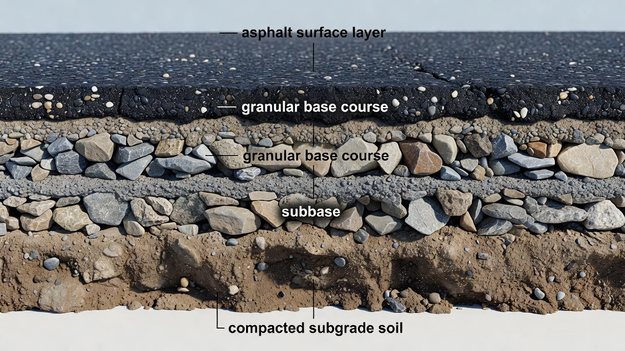
The SN integrates three fundamental pavement design inputs: the thickness of each layer (D), the relative strength of each layer material expressed as a layer coefficient (a), and the quality of drainage in each untreated layer expressed as a drainage coefficient (m). The equation SN = a₁D₁ + a₂D₂m₂ + a₃D₃m₃ aggregates these contributions from the surface course (layer 1) downward through the base (layer 2) and subbase (layer 3) into a single structural capacity value.
The significance of the SN extends beyond new design. During pavement condition inspection, the effective SN of an existing pavement — back-calculated from Falling Weight Deflectometer (FWD) deflection data — provides a quantitative measure of structural deterioration. Comparing the effective SN to the original design SN reveals the remaining structural life of the pavement and determines whether overlay rehabilitation is needed.
SN Formula: SN = a₁D₁ + a₂D₂m₂ + a₃D₃m₃
The structural number is calculated using the additive layer formula defined in the AASHTO 1993 Guide:
SN = a₁D₁ + a₂D₂m₂ + a₃D₃m₃ + …
Where each term in the equation corresponds to a single pavement layer, numbered from the top down:
Variable
Description
Units
Typical Range
a₁, a₂, a₃
Layer coefficient (relative strength of material)
dimensionless
0.05 – 0.50
D₁, D₂, D₃
Layer thickness
inches
1 – 24+
m₂, m₃
Drainage modification coefficient
dimensionless
0.40 – 1.40
The formula can be extended to any number of layers (SN = Σ aᵢDᵢmᵢ), but three layers — surface, base, and subbase — are the standard configuration in most flexible pavement designs. The subscript numbering begins at the top of the pavement structure: layer 1 is the asphalt concrete surface course, layer 2 is the base course, and layer 3 is the subbase course. The subgrade soil is not included in the SN calculation because it is accounted for separately in the design equation through the resilient modulus (MR).
The drainage coefficient mᵢ applies only to untreated granular base and subbase layers. The surface asphalt concrete layer and any stabilized or treated layers (cement-treated base, asphalt-treated base) typically use m = 1.0 because these materials are not susceptible to moisture damage in the same way as unbound granular materials.
A typical SN calculation can be illustrated with a standard pavement cross-section. Consider a pavement consisting of 5 inches of HMA surface (a₁ = 0.44), 8 inches of crushed stone base (a₂ = 0.14, m₂ = 1.0), and 10 inches of granular subbase (a₃ = 0.10, m₃ = 0.85):
Each layer’s contribution to the total SN is independent. The surface layer often contributes the largest share because HMA has the highest layer coefficient. In the example above, the 5-inch HMA surface contributes 2.20 (53%) of the total SN of 4.17, while the base contributes 1.12 (27%) and the subbase contributes 0.85 (20%).
The AASHTO flexible pavement design equation solves for the required SN of the total pavement structure. Once the required SN is determined, the designer must select a combination of layer thicknesses, materials, and drainage provisions that satisfy SN = a₁D₁ + a₂D₂m₂ + a₃D₃m₃. The design SN must equal or exceed the required SN — typically within 0.10 of the required value per the NCDOT design procedure.
The design process involves trial thickness selection. The designer begins with a minimum surface thickness (typically 2–4 inches for HMA), selects candidate base and subbase materials with known layer coefficients, assigns drainage coefficients based on expected moisture conditions, and calculates the resulting SN. If the calculated SN is less than required, one or more layer thicknesses must be increased, or higher-quality materials must be specified.
Layer Coefficients (a₁, a₂, a₃)
The layer coefficient (aᵢ) is a dimensionless number that represents the relative structural contribution per unit thickness of a given pavement material. It was originally derived from the AASHO Road Test performance data and is a function of the material’s resilient modulus, which is a more fundamental material property. The higher the layer coefficient, the greater the structural contribution per inch of that material.
The layer coefficient for the HMA surface course (a₁) is the highest of the three layers because asphalt concrete is the strongest and stiffest pavement material. The standard a₁ value for dense-graded hot mix asphalt used in the AASHO Road Test is 0.44, which corresponds to a resilient modulus of 450,000 psi (3.1 GPa) at 70°F (21°C). The AASHTO design guide provides Figure 11.27, a chart that relates HMA layer coefficient to resilient modulus. An approximate formula derived from this relationship is:
a₁ = 0.40 + 0.031 × log(E₁/10⁵)
Where E₁ is the HMA resilient modulus in psi. For modified asphalt mixtures with higher stiffness, a₁ values up to 0.50 may be used, but the AASHTO guide cautions that using moduli greater than 450,000 psi is accompanied by increased susceptibility to thermal cracking and fatigue cracking, so the higher values should be applied carefully.
The layer coefficient for the untreated granular base course (a₂) is substantially lower because crushed stone and gravel have lower stiffness than HMA. The standard a₂ value from the AASHO Road Test is 0.14, corresponding to a base resilient modulus of 30,000 psi (207 MPa). The following empirical equation relates a₂ to the base resilient modulus (E₂) for untreated granular materials:
a₂ = 0.249 × log(E₂) — 0.977
The modulus of untreated granular materials depends on the stress state (confining pressure), which increases with depth. A typical E₂ range is 20,000 to 40,000 psi. For stabilized base materials, the layer coefficients are higher: cement-treated granular base a₂ = 0.20, asphalt-treated base Class I a₂ = 0.34, and bituminous-treated aggregate base a₂ = 0.23.
The layer coefficient for the subbase course (a₃) is the lowest of the three layers, reflecting the lower stiffness of granular subbase materials. The standard a₃ value from the AASHO Road Test is 0.10 to 0.11, corresponding to a subbase resilient modulus of approximately 15,000 psi (104 MPa).
The following table summarizes typical layer coefficient values from the AASHTO 1993 Guide and various state agencies:
Pavement Layer Material
Layer Coefficient (a)
Minimum Thickness (inches)
HMA with Type A aggregate
0.44
2
HMA with Type B aggregate
0.40
2
Asphalt-treated base Class I
0.34
4
Asphalt-treated base Class II
0.26
4
Bituminous-treated aggregate base
0.23
6
Cement-treated granular base
0.20
6
Soil-cement base
0.15
6
Crushed stone base
0.14
6
Macadam stone base
0.12
6
Portland cement concrete base (new)
0.50
—
Old Portland cement concrete
0.40
—
Crack and seated PCC
0.25 – 0.30
—
Cold in-place recycled
0.22 – 0.27
—
Soil-cement subbase
0.10
6
Soil-lime subbase
0.10
6
Granular subbase
0.10
4
Soil-aggregate subbase
0.05
4
Layer coefficients can be determined by three methods: (1) from test roads or satellite sections as done in the AASHO Road Test, (2) from correlations with resilient modulus using the AASHTO charts, or (3) from established agency policy tables. Most state highway agencies adopt standard layer coefficients for their commonly used materials as a matter of design policy, which ensures consistency across projects.
The resilient modulus testing approach provides the most fundamental basis for layer coefficient selection. The AASHTO T 307 standard test method measures the resilient modulus of asphalt concrete, untreated base, and subbase materials under cyclic loading conditions that simulate traffic. The resulting modulus values are then entered into the AASHTO correlation charts to obtain the corresponding layer coefficients.
Drainage Coefficients (mᵢ)
The drainage modification coefficient (mᵢ) is a multiplier applied to the base and subbase layer coefficients to account for the effect of moisture conditions on the structural performance of untreated granular layers. Water trapped within the pavement structure is one of the primary causes of pavement failure, contributing to loss of strength in unbound materials, pumping of fines, and accelerated deterioration under traffic loading.
The AASHTO 1993 Guide defines the drainage coefficient based on two factors: the quality of drainage (time required to drain the pavement to 50% saturation) and the percentage of time the pavement is exposed to moisture levels approaching saturation.
The drainage quality is classified into five categories:
Drainage Quality
Time to Drain to 50% Saturation
mᵢ Value (Less than 1% time)
mᵢ Value (1% to 5% time)
mᵢ Value (5% to 25% time)
Excellent
2 hours
1.40 – 1.20
1.35 – 1.15
1.30 – 1.10
Good
1 day
1.35 – 1.15
1.25 – 1.05
1.15 – 0.95
Fair
7 days
1.25 – 1.05
1.15 – 0.95
1.00 – 0.80
Poor
1 month
1.15 – 0.95
1.00 – 0.80
0.85 – 0.65
Very Poor
Does not drain
1.05 – 0.85
0.85 – 0.65
0.65 – 0.45
The three moisture exposure columns represent: Less than 1% of the time the pavement is exposed to near-saturation moisture, 1% to 5%, and 5% to 25%. The higher mᵢ values reflect better drainage conditions that improve structural contribution, while lower values penalize poor drainage.
A drainage coefficient of 1.00 represents fair drainage with moderate moisture exposure and has no effect on the SN calculation. Values greater than 1.00 (up to 1.40) increase the effective SN by rewarding good drainage that keeps the granular layers dry and strong. Values less than 1.00 (down to 0.45) reduce the effective SN, requiring thicker pavement layers to compensate for moisture-weakened support.
The drainage coefficient applies only to untreated granular base and subbase layers. The HMA surface layer and any stabilized or bound layers (cement-treated, asphalt-treated, or lean concrete) are considered impermeable or not moisture-susceptible and are assigned m = 1.0. Some state agencies further restrict the maximum mᵢ value; for example, the City of Gillette, Wyoming standards specify that unless an edge drain is provided, the drainage coefficient shall not be greater than 1.00.
The selection of appropriate drainage coefficients requires engineering judgment about the site-specific conditions. Key considerations include: the presence of edge drains or underdrains, the permeability of the granular layers, the annual rainfall and groundwater table elevation, the pavement cross-slope and drainage path length, and the quality of construction compaction. Well-drained pavements with edge drains can achieve m = 1.20 to 1.40, while pavements in wet climates with poor side drainage may be penalized with m = 0.70 to 0.80.
Required SN from the AASHTO Design Equation
The required SN is the value that must be built into the pavement structure to carry the predicted traffic loading over the design life with acceptable serviceability loss. It is determined by solving the AASHTO 1993 flexible pavement design equation, which has the following form:
W₁₈ = predicted number of 18-kip (80 kN) ESALs over the design life
ZR = standard normal deviate for a given reliability level
S₀ = combined standard error (overall standard deviation)
SN = structural number being solved for
ΔPSI = serviceability loss (po — pt)
MR = subgrade resilient modulus (psi)
4.2 = initial serviceability index (po) for flexible pavements
1.5 = terminal serviceability index (pt) for design purposes
The equation is not directly solvable for SN because SN appears both inside and outside logarithmic and exponential terms, requiring iterative trial-and-error solution or the use of the AASHTO design nomograph (Figure 11.25 in the 1993 Guide). The design nomograph provides a graphical solution that is most convenient for determining SN. If W₁₈ is the unknown, the equation can be solved directly.
The standard inputs to the equation are:
Input Variable
Typical Values
Notes
W₁₈ (ESALs)
10⁵ — 5 × 10⁷
Traffic over design life
Reliability (R)
80% — 99%
95% for arterials; 80-88% for collectors/local
ZR
-0.841 to -2.326
Corresponds to R = 80% to 99%
S₀
0.40 — 0.50
0.45 commonly used for flexible pavement
ΔPSI
1.5 — 2.5
po=4.2 minus pt (1.5-2.5 typical)
MR (subgrade)
3,000 — 15,000 psi
Determined from CBR or laboratory testing
The reliability level accounts for uncertainty in traffic prediction, material variability, and construction quality. For arterial highways, R = 99% (ZR = -2.326) is commonly specified, while collector streets use R = 88% (ZR = -1.270) and local streets use R = 80% (ZR = -0.841). Higher reliability requires a higher SN for the same traffic and subgrade conditions.
The overall standard deviation (S₀) reflects the combined uncertainty in traffic loading predictions and pavement performance predictions. The AASHTO guide recommends S₀ = 0.35 to 0.50 for flexible pavements, with 0.45 being the most commonly used value for design.
The serviceability loss (ΔPSI) represents the difference between the initial serviceability index (po = 4.2 for flexible) and the terminal serviceability index (pt). The terminal serviceability represents the lowest acceptable condition before the pavement requires rehabilitation. Typical pt values are: 2.50 for arterials, 2.25 for collectors, and 2.00 for local roads.
The subgrade resilient modulus (MR) is a critical input. It is determined through laboratory testing (AASHTO T 307) or correlations with California Bearing Ratio (CBR) using the relationship MR = 2555 × CBR⁰·⁶⁴. The effective roadbed soil resilient modulus accounts for seasonal variations in subgrade strength due to freeze-thaw cycles and moisture changes. The AASHTO guide provides a procedure that divides the year into monthly periods, assigns seasonal moduli, computes the relative damage factor (uf) for each period using:
uf = 1.18 × 10⁸ × MR⁻²·³²
The average relative damage across all periods is then used to determine the effective MR — the single equivalent modulus that would produce the same cumulative damage if used year-round. This effective MR is often significantly lower than the normal laboratory modulus because the subgrade is weakest during spring thaw, when most damage occurs.
Effective SN of Existing Pavement (Back-calculated from FWD)
The effective structural number (SN_eff) of an existing in-service pavement is determined through non-destructive deflection testing, most commonly using the Falling Weight Deflectometer (FWD). The FWD applies a dynamic impulse load to the pavement surface — typically 9,000 to 27,000 lbf (40 to 120 kN) — simulating the load of a moving truck axle, and measures the resulting surface deflections at multiple radial distances from the load center using geophones or seismometers.
The backcalculation process involves the following steps:
Deflection measurement: FWD collects deflection basins at test points spaced at regular intervals (typically 50 to 200 feet depending on project-level vs. network-level testing)
Backcalculation analysis: Using software such as EVERCALC, MODCOMP, or ELMOD, the measured deflection basin is matched to a theoretical deflection basin computed from layered elastic theory
Layer modulus determination: The backcalculation software estimates the in-situ elastic modulus of each pavement layer (HMA, base, subbase) and the subgrade by iteratively adjusting moduli until the theoretical deflections match the measured deflections
Effective SN computation: The back-calculated layer moduli are used to compute the in-place layer coefficients, which are then summed to obtain the effective SN
The relationship between the back-calculated layer modulus and the layer coefficient follows the AASHTO correlation charts. For the HMA layer, the resilient modulus (E₁) is determined at the FWD testing temperature and then corrected to the standard reference temperature of 70°F (21°C) using temperature correction factors. The layer coefficient a₁ is obtained from the corrected modulus using the AASHTO Figure 11.27 or the empirical correlation equation.
For the base and subbase layers, the back-calculated moduli (E₂, E₃) are used with the appropriate correlation equations to determine a₂ and a₃. The drainage coefficients (m₂, m₃) are selected based on the observed drainage conditions at the test site.
The effective SN is then:
SN_eff = a₁D₁ + a₂D₂m₂ + a₃D₃m₃
Where D₁, D₂, D₃ are the measured layer thicknesses from pavement cores or construction records.
Research by the FHWA Long-Term Pavement Performance (LTPP) program has shown that the effective SN of an existing pavement decreases over time as the pavement deteriorates. The rate of SN loss depends on traffic loading, environmental conditions, and the quality of construction. Typical SN loss rates range from 0.01 to 0.05 per year for well-performing pavements, but can be significantly higher for pavements with premature distress.
The effective SN is a key input for pavement management systems at both the network and project levels. At the network level, SN_eff data from routine FWD testing provides an objective measure of structural capacity that can be sorted, ranked, and trended over time to identify sections requiring rehabilitation. At the project level, SN_eff is used directly in overlay design computations.
The AASHTO R 69 (formerly FHWA protocol) provides standard procedures for using FWD deflection testing to evaluate the structural condition of pavements for overlay design. The protocol specifies test load levels, deflection sensor spacing, temperature correction procedures, and backcalculation acceptance criteria.
SN Deficiency and Overlay Design
The structural deficiency of an existing pavement is quantified by comparing the effective SN (SN_eff) to the required SN (SN_required) for the future traffic. The SN deficiency (also called SN deficit) is:
SN_deficiency = SN_required — SN_eff
If the SN deficiency is positive, the existing pavement does not have sufficient structural capacity to carry the projected future traffic, and an overlay (or other rehabilitation) is needed to restore structural capacity. If SN_eff exceeds SN_required, the pavement has adequate structural capacity and may only need surface treatments or preventive maintenance.
The required overlay thickness (D_overlay) is determined using the SN deficiency:
D_overlay = SN_deficiency / a_overlay
Where a_overlay is the layer coefficient of the overlay material — typically 0.44 for HMA overlay. For example, if SN_required = 5.5 and SN_eff = 3.5, the SN deficiency is 2.0. Using an HMA overlay with a_overlay = 0.44, the required overlay thickness is:
D_overlay = 2.0 / 0.44 = 4.5 inches
The AASHTO 1993 Guide provides two methods for determining the effective structural number for overlay design: the Nondestructive Deflection Testing method (using FWD) and the Condition Survey method (using visual distress and coring). The deflection testing method is more reliable because it directly measures the structural response of the pavement, while the condition survey method relies on engineering judgment to reduce the original design SN based on observed distress.
The overlay design equation also accounts for the fact that the existing pavement structure continues to contribute to the structural capacity even after overlay construction. The existing pavement must still be in reasonable condition to serve as a foundation for the overlay. The SN_eff values used in overlay design should reflect the remaining structural value of each existing layer, not simply the original design SN.
AASHTO overlay design uses the following approach:
Determine SN_required for future traffic and subgrade conditions
Determine SN_eff of the existing pavement from FWD backcalculation
Compute SN_overlay = SN_required — SN_eff (adjusted for potential fatigue of existing HMA)
Convert SN_overlay to overlay thickness: D_overlay = SN_overlay / a_overlay
Some state agencies apply a minimum overlay thickness regardless of the computed SN deficiency, typically 1.5 to 2.0 inches, to ensure adequate construction quality and to address surface distress that may not be fully captured by the structural analysis.
SN and Inspection Condition
The relationship between the Structural Number and visual pavement condition is not direct but is well-established through pavement management research. A pavement with high visual distress may still have adequate structural capacity (measured by SN_eff), and conversely, a pavement with good surface condition may have low structural capacity due to subsurface deterioration that has not yet manifested at the surface.
During pavement condition inspection, the following relationships between SN and observed condition are recognized:
Alligator (fatigue) cracking is the surface manifestation of structural fatigue in the HMA layer. When the tensile strain at the bottom of the HMA layer exceeds the fatigue endurance limit of the asphalt, repeated loading produces bottom-up cracking that propagates to the surface as interconnected alligator cracks. The extent of alligator cracking in the wheel path is directly correlated with the number of ESALs applied relative to the structural capacity of the pavement. A high-severity alligator cracking (LTPP severity levels 2-3) covering more than 25% of the wheel path area strongly indicates that SN_eff is below SN_required.
Rutting (permanent deformation) in the wheel path is related to structural capacity loss when it results from deformation in the subgrade or unbound layers. Surface rutting of 0.5 inches or greater accompanied by pavement heave adjacent to the wheel path indicates structural rutting (subgrade shear failure) that reduces the effective SN.
Patching and previous repairs are considered indicators of structural capacity loss. Large patched areas (>10% of slab or lane area) suggest that the pavement has undergone structural failure in those locations and the effective SN should be adjusted downward accordingly.
International Roughness Index (IRI) increases as structural condition deteriorates, but the correlation is weak at the project level because IRI is influenced by many factors besides structural capacity.
The standard protocol used by many state DOTs and airport authorities is to calculate an adjusted SN based on visual condition during Pavement Condition Index (PCI) surveys. The AASHTO condition survey method for overlay design provides reduction factors that are applied to the original design SN based on the extent and severity of observed distress:
Distress Type
Condition
SN Reduction Factor
No significant distress
Good
0.90 — 1.00
Moderate fatigue cracking (<20% area)
Fair
0.70 — 0.85
Extensive fatigue cracking (>20% area)
Poor
0.50 — 0.70
Structural rutting (>0.5 in)
Poor
0.50 — 0.65
Severe patching (>20% area)
Poor
0.40 — 0.60
These reduction factors provide a visibility-based estimate of SN_eff when FWD testing is not available, but they are significantly less accurate than FWD backcalculation. The standard deviation of the condition-based SN estimate compared to FWD-based SN can be as high as 0.5 to 0.8 SN units.
For comprehensive pavement evaluation, the combination of FWD deflection testing (for structural capacity) and PCI survey (for surface condition) provides the most complete picture. Pavement sections with both low SN_eff and high distress severity are candidates for structural overlays or reconstruction, while sections with adequate SN but poor surface condition may only need surface treatments or milling and overlay.
SN in Airport Flexible Pavement Design
The Structural Number concept from the AASHTO highway method has limited direct application to airport flexible pavement design, which uses the FAA FAARFIELD (FAA Airport Pavement Design Program) method based on layered elastic analysis. However, the underlying principle of expressing structural capacity as a summation of layer contributions is conceptually similar to the FAA approach.
The ICAO ACN-PCN (Aircraft Classification Number — Pavement Classification Number) system uses a standardized numerical rating of pavement structural strength. The PCN is determined through a technical evaluation that involves either: (1) using the FAA CBR design curves (for flexible pavements), (2) using the FAA FAARFIELD program, or (3) using the ACN method from ICAO Aerodrome Design Manual Part 3.
For flexible airfield pavements designed using the FAA CBR method (which was the standard before FAARFIELD was mandated in 2009), the pavement thickness design curves relate total pavement thickness above the subgrade to:
Aircraft weight and configuration (landing gear type, tire pressure)
Annual departures (traffic frequency)
Subgrade CBR (strength)
The FAA CBR method’s output is a total pavement thickness above the subgrade, expressed as a combined structure. While this is not identical to the AASHTO SN, the FAA design procedure’s equivalent thickness concept (converting various base types to equivalent hot mix asphalt thickness using equivalency factors) is functionally similar to the SN layer coefficient approach.
The equivalency factors used by FAA (per AC 150/5320-6G) for converting base and subbase layers to equivalent HMA thickness include:
Base Material
Equivalency Factor
HMA surface/base
1.0
P-208 aggregate base
0.75
P-209 crushed aggregate base
0.75
P-304 cement-treated base
0.75
P-306 econocrete base
0.67
These equivalency factors are analogous to the ratio of layer coefficients (a₂/a₁, a₃/a₁) in the AASHTO method. For example, if a₁ = 0.44 for HMA and a₂ = 0.14 for aggregate base, the equivalency ratio is 0.14/0.44 = 0.32, meaning one inch of aggregate base is structurally equivalent to about 0.32 inches of HMA. The FAA’s equivalency factor of 0.75 for aggregate base differs from this ratio because the FAA method accounts for the heavier loads and different failure criteria of aircraft loading.
The FAARFIELD method (FAA AC 150/5320-6G, since 2009) uses a three-dimensional layered elastic finite element analysis (LEAF) to compute stresses and strains in the pavement structure under aircraft loading. The cumulative damage factor (CDF) approach compares the computed critical strains to allowable strains derived from laboratory fatigue and rutting tests. FAARFIELD does not use the SN concept, but the output is a set of layer thicknesses that together provide the required structural capacity.
For airfield pavement evaluation, some agencies have adapted the AASHTO SN approach to provide a relative structural index for network-level pavement management. The effective SN of an airfield pavement can be estimated from FWD testing using the same backcalculation principles as highway pavements, and the SN deficiency approach provides a rational basis for prioritizing rehabilitation needs. However, the overlay thickness must be verified using the FAA FAARFIELD procedure before final design.
The structural condition index (SCI) and pavement condition index (PCI) used in airfield pavement management combine structural capacity (FWD-based) with surface condition (visual inspection) to provide a comprehensive evaluation. The interaction between SN, PCI, and remaining life is assessed through the airport pavement management system, which uses these indices to prioritize maintenance and rehabilitation projects.
AASHTO 1993 vs MEPDG: The Evolution Beyond SN
The AASHTO 1993 Guide and the Mechanistic-Empirical Pavement Design Guide (MEPDG), implemented through the AASHTOWare Pavement ME software, represent two fundamentally different approaches to flexible pavement design. The Structural Number concept is central to the 1993 method but is not used in the MEPDG approach.
Aspect
AASHTO 1993
MEPDG (Pavement ME)
Basis
Empirical (AASHO Road Test, 1958-60)
Mechanistic-empirical (layered elastic + transfer functions)
The AASHTO 1993 method produces a single SN value that must be translated into layer thicknesses through the SN = Σ aᵢDᵢmᵢ formula. It does not directly predict specific distress types. The terminal serviceability index (pt) is the single performance criterion — when the pavement reaches pt, rehabilitation is needed regardless of the type of distress that caused the serviceability loss.
The MEPDG evaluates multiple performance criteria simultaneously. The design is iterated until all predicted distresses (rutting, fatigue cracking, thermal cracking, and IRI) remain below user-specified thresholds at the target reliability level. The MEPDG does not use the SN concept because it treats each layer’s properties independently and evaluates their combined response using mechanistic analysis rather than empirical summation.
The primary advantages of the MEPDG over the AASHTO 1993 method are:
Climate integration: The MEPDG uses hourly climate data (temperature, precipitation, wind speed, solar radiation) from over 800 weather stations to model seasonal changes in material properties and moisture conditions within the pavement structure. The 1993 method only adjusts the subgrade resilient modulus seasonally.
Traffic spectra: Rather than reducing traffic to a single ESAL count, the MEPDG uses axle load spectra — the full distribution of single, tandem, tridem, and quad axle loads by weight category. This provides a more accurate representation of traffic damage, particularly for routes with significant overload violations or unusual axle configurations.
Material-specific distress models: The MEPDG uses different distress models for different material types (dense-graded HMA, SMA, OGFC, various base types) with material-specific calibration coefficients derived from LTPP data.
Enhanced reliability: Reliability targets are applied separately to each distress type rather than as a single global factor applied to the loading.
However, the AASHTO 1993 method remains in widespread use for several practical reasons:
Simplicity: The method requires far fewer inputs and can be applied using nomographs or simple spreadsheets
Familiarity: Most pavement engineers trained in the US are familiar with the 1993 method
Calibration: The MEPDG requires local calibration for each region’s materials and climate to achieve reliable results
Institutional inertia: Many state agencies have developed design catalogs, standard specifications, and construction acceptance criteria based on the 1993 method
Data availability: The 1993 method requires only ESALs, MR, and basic material type, while the MEPDG requires detailed material testing (dynamic modulus, creep compliance) that may not be available for all projects
The transition from the AASHTO 1993 approach to the MEPDG has been gradual but steady. As of 2023, approximately 25 state DOTs have adopted or were in the process of adopting the MEPDG for routine design, while others use it for specific project types (high-volume roads, unusual materials, or critical facilities) while continuing to use the 1993 method for standard designs.
For pavement condition inspection and evaluation, the AASHTO 1993 SN concept remains valuable because the effective SN from FWD testing provides a direct and intuitive measure of remaining structural capacity that can be easily compared to design requirements. The MEPDG does not provide an equivalent single index of structural capacity — instead, it evaluates whether the predicted distresses remain below thresholds. For network-level pavement management, the SN concept remains the standard approach for ranking structural capacity across a pavement network.
Frequently Asked Questions
Typical Structural Number values vary widely depending on traffic loading and subgrade conditions. A low-volume road may have an SN of 2.0 to 3.0, while a major interstate highway with heavy truck traffic may require an SN of 5.0 to 7.0 or higher. For example, a pavement designed for 5 million ESALs on a subgrade with MR = 5,000 psi at 95% reliability typically yields an SN around 5.0. Airport flexible pavements for heavy aircraft can require SN values exceeding 10.0, depending on the aircraft classification number (ACN) and subgrade strength.
SN is calculated using the formula SN = a1D1 + a2D2m2 + a3D3m3, where a1, a2, a3 are the layer coefficients for the surface, base, and subbase respectively, D1, D2, D3 are the layer thicknesses in inches, and m2, m3 are the drainage modification coefficients for the base and subbase layers. For example, a 4-inch HMA surface (a1 = 0.44), 8-inch crushed stone base (a2 = 0.14, m2 = 1.0), and 12-inch granular subbase (a3 = 0.10, m3 = 0.90) yields SN = (0.44 × 4) + (0.14 × 8 × 1.0) + (0.10 × 12 × 0.90) = 1.76 + 1.12 + 1.08 = 3.96.
The required SN is the structural number determined from the AASHTO design equation that a pavement must have to sustain the design traffic loading over its design life. The effective SN (SN_eff) is the actual structural capacity of an existing in-service pavement, typically determined through falling weight deflectometer (FWD) deflection testing and backcalculation analysis. The difference between the required SN and the effective SN (SN_deficiency = SN_required - SN_eff) is used to determine the thickness of overlay needed for pavement rehabilitation.
The AASHTO 1993 method uses an empirical equation based on the AASHO Road Test (1958-1960) and produces a single Structural Number value as the design output. The Mechanistic-Empirical Pavement Design Guide (MEPDG / Pavement ME) uses mechanistic layered elastic analysis to compute stresses, strains, and deflections, then applies empirical transfer functions to predict specific distresses (fatigue cracking, rutting, thermal cracking). The MEPDG does not use the SN concept but instead evaluates individual layer moduli, thicknesses, and distress predictions over the design life. The MEPDG provides a more detailed analysis that accounts for climate, material properties, and traffic spectra, whereas the 1993 AASHTO method is simpler and remains widely used due to its established familiarity.
The structural number concept is primarily a highway pavement design parameter from the AASHTO method. However, the ICAO ACN-PCN method and the FAA FAARFIELD design procedure for airport pavements use different approaches: the ACN-PCN system uses a standard numerical rating for pavement strength, and FAARFIELD uses layered elastic finite element analysis (LEAF) with cumulative damage factors (CDF). While the FAA CBR method for flexible airfield pavements has some conceptual similarities to the AASHTO SN approach, the FAARFIELD method has been the standard for US airport design since 2009. The SN concept may still be referenced by some agencies for airfield pavement evaluation at the network level.
The standard layer coefficient for dense-graded hot mix asphalt (HMA) used in the AASHO Road Test is 0.44, corresponding to a resilient modulus of approximately 450,000 psi (3.1 GPa) at 70°F (21°C). Higher modulus values up to 0.50 may be used for modified asphalt mixtures, but caution is advised because higher stiffness is associated with increased susceptibility to thermal and fatigue cracking. The AASHTO design guide provides a chart (Figure 11.27) relating HMA layer coefficient to resilient modulus at 70°F. Many state highway agencies adopt the standard a1 = 0.44 as policy.
Assess pavement structural capacity with precision
TarmacView helps airport and highway pavement managers calculate, track, and compare effective Structural Numbers against design requirements. Schedule a demo to see how automated FWD data analysis streamlines structural evaluation.
Pavement thickness design determines the layer thicknesses required to support traffic loads over the design life. Methods include empirical (AASHTO 1993; FAA C...
Traffic loading data — vehicle classifications, axle loads, and counts — is a primary input for pavement structural design and determines the rate of pavement c...
FWD deflection data analysis processes the measured deflection basin from FWD testing to back-calculate the elastic modulus of each pavement layer (HMA, base, s...
38 min read
Pavement Testing
Structural Evaluation
+3
Cookie Consent We use cookies to enhance your browsing experience and analyze our traffic. See our privacy policy.