Domain Adaptation
Domain adaptation adapts machine learning models trained on a source domain — such as specific pavement types, lighting conditions, or datasets — to perform rel...
35 min read
Technology
Machine Learning
+2
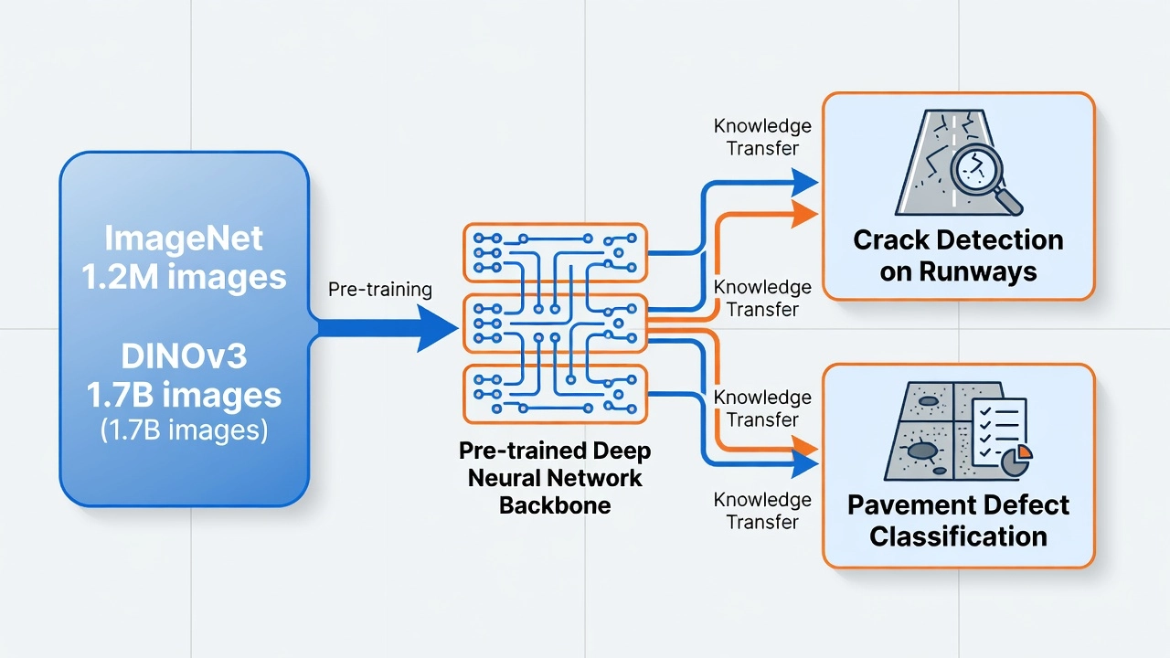
Transfer learning applies knowledge from a model pre-trained on large general datasets (ImageNet 1.2M images, DINOv3 on 1.7B images) to specialized infrastructure inspection tasks with limited labeled data, such as crack detection, defect classification, and pavement condition assessment. It drastically reduces the amount of task-specific training data needed.
Transfer learning is a machine learning paradigm in which a model developed for one task is reused as the starting point for a model on a second, related task. In computer vision for infrastructure inspection, this involves taking a neural network pre-trained on a large, generic dataset — such as ImageNet with 1.2 million images across 1,000 classes, or Meta DINOv3 self-supervised model trained on 1.7 billion curated images — and adapting it to detect cracks, spalling, rubber deposits, joint deterioration, and other pavement defects using a small fraction of the labeled data that would be required to train from scratch.
Formally, transfer learning is defined as follows: Given a source domain D_S with a learning task T_S, and a target domain D_T with learning task T_T, transfer learning aims to improve the learning of the target predictive function f_T in D_T using knowledge from D_S and T_S, where D_S ≠ D_T and/or T_S ≠ T_T. This formal definition, established by Pan and Yang in their 2010 survey on transfer learning, distinguishes the paradigm from related approaches like multi-task learning (where both tasks are learned simultaneously) and domain adaptation (where the task is identical but the data distribution changes).
Three distinct but related terms are often conflated in practice. Pre-training is the initial training phase where a model is trained on a large-scale dataset, typically requiring thousands of GPU-hours for modern architectures — this is now an industrial-scale operation performed by organizations like Meta, Google, and OpenAI. Transfer learning is the broad paradigm of reusing knowledge from one domain or task in another, encompassing multiple strategies beyond simple weight initialization. Fine-tuning is the most common transfer learning technique, where pre-trained weights are adjusted on the target dataset through continued training, either partially (with frozen layers) or fully, using a reduced learning rate to prevent catastrophic forgetting of pre-trained knowledge.
The fundamental reason transfer learning works in computer vision is the hierarchical nature of learned features in deep neural networks. This hierarchy has been validated through gradient ascent visualizations, activation heatmaps, and feature inversion techniques across both convolutional neural networks (CNNs) and Vision Transformers (ViTs).
Early layers — the first convolutional blocks in CNNs or the initial transformer blocks in ViTs — detect low-level features such as edges (vertical and horizontal), gradients, color blobs, and simple textures. These features are largely domain-agnostic: the edge detectors learned from ImageNet photographs of animals and objects are equally effective at finding crack boundaries in pavement images. Studies using CKA (Centered Kernel Alignment) similarity metrics have shown that early layer representations have 80-90% overlap between natural image domains and infrastructure inspection domains.
Middle layers learn mid-level patterns such as shapes (circles, corners), textures (grids, stripes, grain patterns), and object parts. Some domain-specific adaptation begins at this level — the texture filters tuned to fur and wood grain must be adjusted to respond to asphalt surface texture and concrete aggregate patterns. Activation similarity between domains drops to 50-70% at middle layers.
Late layers — the final transformer blocks or fully-connected classifier layers — learn task-specific, high-level semantic features such as object categories, scene types, and domain-specific patterns. These layers require the most adaptation and are typically the first to be fine-tuned when transferring to a new domain. Activation similarity between domains at late layers drops below 30%, confirming that the majority of domain-specific learning happens here.
This hierarchical understanding directly informs transfer learning strategy. The decision of how many layers to freeze, which learning rates to assign to each layer group, and whether to use progressive unfreezing all derive from the principle that early layers are universal, middle layers are partially transferable, and late layers are task-specific.
Infrastructure inspection domains — particularly airport runway pavement assessment — present several characteristics that make transfer learning essential rather than optional.
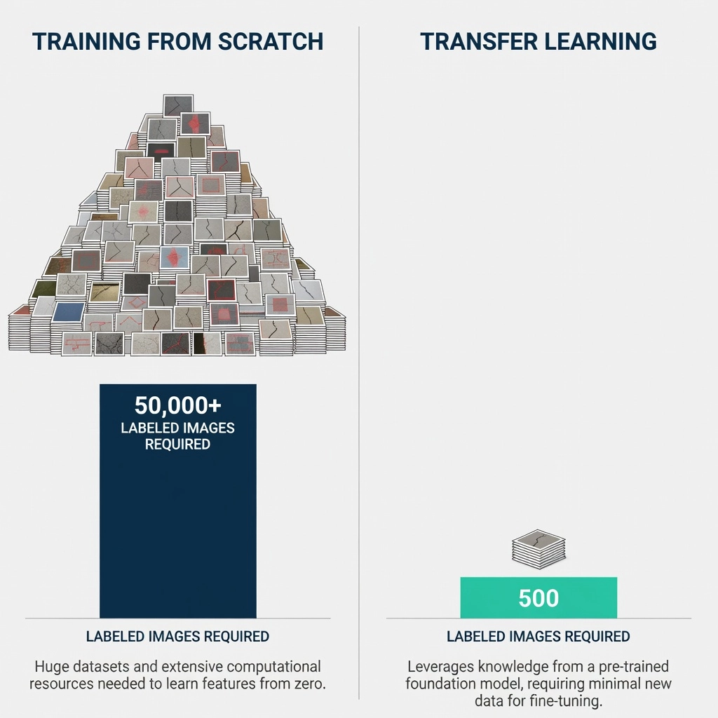
Severe data scarcity is the primary driver. Labeled defect datasets for airport runways are extremely limited in availability and scale. A typical runway crack detection project might have access to 500-5,000 labeled images, which is two to three orders of magnitude less than what is needed for training a deep neural network from scratch. Public datasets for road pavement cracks exist (CQU-BPDD with 60,088 images, RDD2020 with 26,336 images), but runway-specific datasets with pixel-level annotations for defects like rubber deposits, joint spalling, and fuel spill damage are predominantly proprietary and small.
High annotation cost compounds the scarcity problem. Pixel-level semantic segmentation of pavement defects — where each pixel in an image must be labeled as belonging to a specific defect category or as normal pavement — requires trained inspectors with knowledge of distress identification manuals. Annotating a single high-resolution runway image (20-50 megapixels) can take 15-60 minutes for a trained professional. At typical labeling costs of $30-60 per hour, building a dataset of 5,000 labeled images represents an investment of $37,500-300,000.
Class imbalance is a universal challenge in infrastructure inspection. Normal pavement constitutes more than 95% of pixel area in most runway images. Defects — cracks, spalling, rubber deposits — occupy a tiny fraction of the image. Standard loss functions like cross-entropy are dominated by the majority class, causing models to learn to predict “normal pavement” for every pixel. Transfer learning mitigates this by providing pre-trained feature representations that are already sensitive to visual anomalies and boundaries.
Safety-critical application demands high accuracy and reliability. Missed defects (false negatives) on runways have direct safety implications for aircraft operations — an undetected structural crack can propagate under load and lead to pavement failure during landing or takeoff. Transfer learning enables models to reach operational accuracy thresholds with the limited data available, making AI-assisted runway inspection practically feasible within current regulatory frameworks.
| Challenge | Impact Without Transfer Learning | Mitigation Through Transfer Learning |
|---|---|---|
| Data scarcity | Requires 50,000-100,000 labeled images | Works with 200-5,000 images (10-250x reduction) |
| Annotation cost | $37,500-300,000 per dataset | $1,500-30,000 per dataset |
| Class imbalance | Model predicts majority class (normal pavement) | Pre-trained features already sensitive to anomalies |
| Safety-critical accuracy | Insufficient accuracy with limited data | Achieves 70-85% mIoU with 500-1,500 images |
ImageNet, introduced by Deng et al. in 2009, remains the most widely used dataset for vision pre-training despite the emergence of larger and more specialized alternatives. The ImageNet-1K subset used in the ILSVRC 2012 challenge contains approximately 1.28 million training images distributed across 1,000 mutually exclusive object classes, with roughly 1,300 images per class on average. The full ImageNet-21K dataset contains approximately 14.2 million images across 21,841 WordNet synsets.
Research by Huh, Agrawal, and Efros (2016) in their paper “What makes ImageNet good for transfer learning?” established several key findings that remain relevant. Pre-training with only half the ImageNet data — 500 images per class instead of 1,300 — achieves 98% of the transfer learning benefit, suggesting diminishing returns to dataset size beyond a threshold. The diversity of classes matters more than the raw number of classes: the 1,000 ImageNet-1K classes span a wide visual spectrum including animals, objects, scenes, and textures, which is what gives the pre-trained features their generality. Features from the middle layers of a pre-trained network transfer best — the first few layers are too generic (pure edge detectors) and the last few are too specific (tuned to ImageNet class boundaries).
Ridnik et al. (2021) demonstrated that ImageNet-21K pre-training provides consistent improvements over ImageNet-1K across downstream tasks including classification, detection, and segmentation, for architectures ranging from large models (TResNet-L) to mobile-oriented (MobileNetV3). For Vision Transformers specifically, ImageNet-21K pre-training provides a notable boost over ImageNet-1K, though the gap narrows with larger self-supervised models.
Meta DINO (Distillation with No Labels) family represents the current state of the art in self-supervised vision transformers. The progression from DINOv1 through DINOv3 illustrates the dramatic scaling of self-supervised learning in recent years.
| Aspect | DINOv1 (2021) | DINOv2 (2023) | DINOv3 (2025) |
|---|---|---|---|
| Training data | ImageNet-1K (~1.2M images) | LVD-142M (142M curated images) | LVD-1689M (~1.7B curated images) |
| Teacher model | ViT-B/8 (307M params) | ViT-g (1.1B params) | ViT-7B (7B params) |
| Key innovation | Self-distillation, momentum teacher | Sinkhorn-Knopp centering, KoLeo regularizer | Gram Anchoring, RoPE embeddings |
DINOv3 architecture and training details scale self-supervised learning to an unprecedented level. The data curation pipeline starts from approximately 17 billion social media images, which after deduplication, quality filtering, and diversity curation yields the LVD-1689M dataset of 1.7 billion images. The model family includes Vision Transformer variants ranging from ViT-S (21 million parameters) to ViT-7B (7 billion parameters), plus ConvNeXt variants optimized for memory-constrained environments.
Key training innovations include a simplified training recipe with fixed hyperparameters throughout training; Gram Anchoring that addresses the tradeoff between global and local feature quality; and high-resolution training using RoPE (Rotary Position Embeddings) with stable feature maps demonstrated at resolutions above 4K. For infrastructure inspection, the critical result is DINOv3 exceptional dense feature quality — each image patch carries semantically meaningful information even without fine-tuning.
Self-supervised pre-training (DINOv3, MAE, SimCLR) differs fundamentally from supervised pre-training (ImageNet classification) in that it does not require any human-labeled data. The model learns visual representations by solving pretext tasks — predicting masked patches, contrasting augmented views of the same image, or matching features across student and teacher networks.
For infrastructure inspection, self-supervised pre-training offers several advantages. The features learned are more general because they are not biased toward any particular class taxonomy. Self-supervised models tend to produce stronger dense features (pixel-level and patch-level representations) compared to supervised models, which is critical for segmentation tasks. The ability to continue pre-training on unlabeled target domain images (e.g., 10,000+ unlabeled runway images) allows domain-specific adaptation without any annotation cost.
| Pre-Training Method | Data Requirement | Label Requirement | Dense Feature Quality |
|---|---|---|---|
| ImageNet supervised | 1.2M images | Yes (1,000 classes) | Moderate |
| ImageNet-21K supervised | 14M images | Yes (21K classes) | Good |
| DINOv2 self-supervised | 142M images | No | Good |
| DINOv3 self-supervised | 1.7B images | No | Excellent |
Linear probing, also called feature extraction, freezes all pre-trained backbone weights and trains only a new classification or segmentation head on top of the extracted features. The backbone acts as a fixed feature extractor, converting input images into high-dimensional feature vectors or feature maps. A simple linear classifier or shallow convolutional decoder is trained on these features to perform the target task.
The advantages of linear probing are substantial. It is extremely fast to train — often requiring minutes rather than hours or days. It requires minimal computational resources because gradients are not backpropagated through the backbone. The risk of overfitting is very low because only a small number of parameters (typically 0.1-1% of the total model) are being trained.
The disadvantage is that the frozen features may not be optimally represented for the target domain. If the domain gap is significant — as it is between ImageNet natural images and runway pavement surfaces — the fixed features may miss important domain-specific patterns. For infrastructure inspection, linear probing with DINOv3 on 200 labeled runway images achieves 55-65% mIoU on defect segmentation — a highly useful result considering that training from scratch on the same data would yield below 20% mIoU.
Full fine-tuning updates all model parameters — both backbone and head — on the target dataset. This provides maximum adaptation to the target domain, allowing all layers to adjust their representations to pavement-specific features. The backbone early layers undergo minor adjustments while later layers can change substantially.
The risks of full fine-tuning include overfitting when the target dataset is small (fewer than 5,000 images) and catastrophic forgetting — the phenomenon where the model overwrites useful pre-trained knowledge because the gradients from the target task dominate training. Mitigation strategies include using a reduced learning rate (typically 0.1x to 0.01x of the pre-training learning rate), applying stronger regularization (weight decay of 0.05-0.3, stochastic depth, label smoothing), and employing early stopping based on target validation loss.
The LP-FT strategy, formalized by Kumar et al. (2022) in “When Does Transfer Learning Work?”, combines the advantages of both approaches. First, the backbone is frozen and a linear probe is trained to convergence. Then, the backbone is unfrozen and the entire model is fine-tuned at a reduced learning rate. This two-stage approach prevents the initial random head weights from corrupting the pre-trained backbone — a phenomenon that Kumar et al. demonstrated causes significant performance degradation in standard one-stage fine-tuning.
The LP-FT approach is particularly effective when the target dataset is small and the task differs substantially from the pre-training task. For runway crack detection, LP-FT consistently outperforms both pure linear probing and direct full fine-tuning, recovering 2-5 additional percentage points of mIoU compared to direct fine-tuning.
When a layer is frozen in a neural network, its weights remain fixed during training. No gradients are computed for that layer during backpropagation, which means the layer contributes no weight updates and consumes no gradient computation. Data still flows through the layer in the forward pass, so frozen layers continue to extract features from the input. The freezing mechanism is implemented by setting the requires_grad flag to False for all parameters in the frozen layers in PyTorch, or by excluding frozen variables from the optimizer parameter list in TensorFlow/Keras.
Vision Transformers exhibit different freezing behavior than CNNs due to their self-attention mechanism. Research by Raghu et al. (2021, “Do Vision Transformers See Like CNNs?”) showed that ViTs maintain more global information throughout all layers compared to CNNs, making layer selection for freezing less straightforward.
Strategy A: Full Backbone Freeze — The entire pre-trained backbone is frozen and only the task-specific head is trained. This is appropriate for very small datasets (fewer than 1,000 images) and computationally constrained environments. For DINOv3 with a frozen backbone, a linear probe on 200-500 labeled runway images achieves 55-65% mIoU.
Strategy B: Stage/Block Freezing — Early layers (e.g., first 50% of ViT blocks) are frozen while later layers are fine-tuned. The rationale is that early blocks capture universal features that transfer well across domains. The typical split is freezing the first 6 of 12 ViT-B blocks.
Strategy C: Progressive Unfreezing — Training starts with the backbone fully frozen and only the head training for N epochs. Then the topmost backbone blocks are unfrozen and training continues at a reduced learning rate. This unfreezing process progresses from top to bottom — later blocks unfreeze first because they need the most adaptation, while early blocks remain frozen longest to preserve universal features. Progressive unfreezing prevents catastrophic forgetting by gradually exposing more of the network to the target domain signal.
Strategy D: Layer-wise Learning Rate Decay (LLRD) — All layers remain trainable but with different learning rates. Early layers receive very low learning rates (1e-6 to 1e-5), middle layers receive moderate rates (1e-5 to 5e-5), and late layers plus the head receive the standard rate (1e-4 to 1e-3). Typical decay factors range from 0.8 to 0.95 per transformer block.
| Freezing Strategy | Target Data Required | Parameters Updated | Forgetting Risk | Best Use Case |
|---|---|---|---|---|
| Full backbone freeze | <1,000 images | <1% | None | Tiny datasets, fast deployment |
| Stage/block freezing | 1,000-10,000 | 10-50% | Low | Moderate domain shift |
| Progressive unfreezing | 1,000-10,000 | Gradual | Low-Medium | Significant domain shift |
| LLRD | >5,000 | 100% (different LRs) | Low | Large datasets, full adaptation |
The head of a transfer learning model is the set of layers added on top of the frozen or fine-tuned backbone that perform the target task. The head must be designed to match the output requirements of the specific inspection task.
For classification tasks (is this pavement image cracked or not?), the head is typically a global average pooling layer followed by one or two fully-connected layers ending with a softmax activation over the number of classes. For binary crack detection, this means 2 output neurons. For multi-class defect classification (crack, spalling, rubber deposit, normal), the head has N+1 output neurons where N is the number of defect types.
For semantic segmentation tasks (assign a defect class to every pixel), the head is typically a decoder that upsamples the backbone feature maps back to the original image resolution. Common choices include Feature Pyramid Networks (FPN), U-Net decoders, and DeepLab-style atrous spatial pyramid pooling (ASPP). The TarmacView pipeline uses a lightweight decoder head that maps DINOv3 patch-level features to pixel-level predictions through a series of transposed convolutions and skip connections.
For object detection tasks (locate and classify defects with bounding boxes), the head typically includes both a classification branch and a bounding box regression branch. Architectures like Mask R-CNN, YOLOv8, and DETR can be adapted as detection heads on top of a pre-trained backbone.
The head is always trained from scratch because it has no pre-trained weights — the pre-training dataset output structure (e.g., 1,000 ImageNet classes) does not match the target task output structure (e.g., 5 defect types). The head typically uses a higher learning rate than the backbone — often 10x to 20x higher in LLRD scheduling — because it needs to converge from random initialization while the backbone needs only minor adjustments.
When using linear probing (frozen backbone), the head is the only trainable component. The learning rate for linear probing is typically 0.01 to 0.1, much higher than fine-tuning rates, because there is no risk of corrupting pre-trained weights.
TarmacView implements a three-stage transfer learning pipeline that leverages the complementary strengths of self-supervised pre-training, supervised contrastive learning, and task-specific fine-tuning.
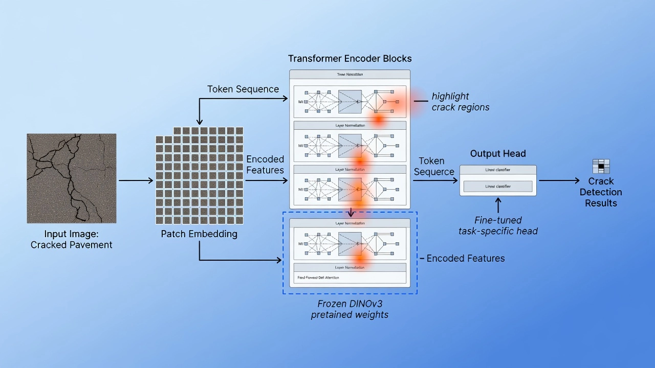
Stage 1: Frozen DINOv3 Backbone — The pipeline starts with a DINOv3 Vision Transformer (ViT-L or ViT-H) pre-trained on 1.7 billion images. The backbone is frozen during initial deployment, meaning no gradients flow through the transformer blocks. Raw runway pavement images are resized to 518x518 pixels, divided into 14x14 patches, and passed through the frozen backbone. The output is a set of dense patch-level feature vectors — 1,372 feature vectors for a 518x518 image — each carrying semantically meaningful information. This stage requires zero labeled data and zero training time per deployment.
Stage 2: Supervised Contrastive Fine-Tuning — A supervised contrastive learning (SupCon) head is attached to the frozen backbone. This head maps the patch-level features into a lower-dimensional embedding space (typically 128-256 dimensions). The SupCon loss pulls feature embeddings of the same class together while pushing embeddings of different classes apart. This fine-tuning uses 200-1,000 labeled runway images and runs for 50-100 epochs. The result is a structured embedding space where defect types form distinct clusters.
Stage 3: Task-Specific Heads — After SupCon fine-tuning, the SupCon head is discarded and replaced with task-specific heads. For pixel-level semantic segmentation, a lightweight decoder head (FPN with 3-4 levels) is trained on the SupCon-fine-tuned backbone features. For PCI estimation, a regression head maps the per-image feature aggregate to a PCI score between 0 and 100.
| Pipeline Stage | Images Required | mIoU (Runway Segmentation) | Training Time |
|---|---|---|---|
| Stage 1 only (frozen DINOv3 + linear probe) | 200-500 | 55-65% | <1 hour on single GPU |
| Stage 1+2 (frozen DINOv3 + SupCon) | 200-1,000 | 65-75% | 2-4 hours on single GPU |
| Stage 1+2+3 (full pipeline) | 500-1,500 | 75-85% | 4-8 hours on single GPU |
| Training from scratch | 50,000+ estimated | <20% | Impractical |
Without transfer learning, each airport deployment would require collecting and labeling 50,000-100,000 images at a cost of $125,000-600,000 per airport. With the three-stage transfer learning pipeline, labeling requirements drop to 200-1,500 images per airport, reducing cost to $500-9,000 per airport. For an airport operator managing 20 airports, transfer learning reduces inspection AI deployment costs from $2.5-12 million to $10,000-180,000 — a reduction of 98-99%.
| Task | From Scratch | With Transfer Learning | Reduction |
|---|---|---|---|
| Image classification (<10 classes) | >10,000 per class | 50-500 per class | 20-200x |
| Fine-grained classification | >50,000 per class | 200-2,000 per class | 25-250x |
| Object detection | >50,000 annotated images | 500-5,000 annotated | 10-100x |
| Semantic segmentation | >100,000 labeled images | 500-10,000 labeled | 10-200x |
| Defect segmentation | >50,000 images | 200-5,000 images | 10-250x |
Without transfer learning, performance follows a log-linear relationship: Performance ≈ α × log(N) + β. Each doubling of dataset size yields diminishing returns. With transfer learning, performance follows an exponential approach to ceiling: Performance ≈ α’ + β’ × (1 - exp(-γN)). The curve saturates much faster, reaching near-asymptotic performance with 1/10th to 1/100th the data.
A frozen DINOv3 backbone with a linear probe on 200 labeled runway patches achieves approximately 55-65% mIoU. Fine-tuning the top 50% of ViT blocks on 1,000-2,000 patches reaches 70-80% mIoU. The full three-stage pipeline on 500-1,500 patches achieves 75-85% mIoU. Training from scratch would require an estimated 50,000-100,000 labeled patches.
The domain gap refers to the statistical difference between the pre-training domain — typically natural images from ImageNet containing animals, objects, and scenes — and the target domain of infrastructure inspection featuring pavement surfaces, cracks, runway markings, and rubber deposits. This gap is the primary reason that transfer learning requires fine-tuning rather than direct application of a frozen model.
Visual domain gap — Pre-training datasets contain natural textures (fur, wood grain, water surfaces) that differ substantially from man-made pavement textures (asphalt aggregate, concrete surface finish). Color distributions differ dramatically: ImageNet spans the full RGB spectrum while pavement images are concentrated in narrow gray, brown, and black ranges.
Semantic domain gap — ImageNet classes include “pavement” as a background context but not as a primary object of interest. Crack detection requires understanding of anomalous linear features against uniform texture — a visual skill not explicitly learned from natural images.
Quantification — Chen et al. (2023) measured that pavement defect datasets have 2-3x larger Frechet Inception Distance (FID) from ImageNet than standard fine-grained classification datasets.
Intermediate domain pre-training — Pre-train on road pavement datasets before fine-tuning on runway data. Road datasets include CQU-BPDD (60,088 images), RDD2020 (26,336 images), Crack500 (500 images), and CFD (6,000 images). This two-step transfer reduces the domain gap at each step.
Self-supervised continued pre-training — Use DINOv3 on unlabeled runway images (10,000+ if available) to learn domain-specific features before fine-tuning with labels.
Data augmentation bridging — Apply augmentations that simulate pavement-like visual conditions. Grayscale conversion removes color as a confounding variable. Elastic transforms simulate crack deformation. Random augmentations improve robustness.
| Domain Gap Dimension | Magnitude | Primary Mitigation |
|---|---|---|
| Visual appearance (texture, color) | Large | Self-supervised continued pre-training on target domain |
| Object scale | Large | Multi-resolution training, pyramid pooling |
| Semantic structure | Large | Intermediate domain pre-training on road datasets |
| Capture conditions | Moderate | Data augmentation, BN statistics recomputation |
Road pavement crack detection is a more mature field with larger, more diverse public datasets than runway inspection. A 2025 USDOT/RITA study explicitly tested road-to-runway transfer using dashcam imagery. Direct road-to-runway transfer achieved approximately 40-50% of fully-supervised runway performance. Road pre-training followed by runway fine-tuning with 500 images achieved >85% of fully-supervised performance with 5,000 runway images. The improvement over ImageNet-only pre-training was 5-15% mIoU on runway defect segmentation.
| Aspect | Road Pavement | Airport Runway Pavement |
|---|---|---|
| Primary material | Asphalt (HMA) | High-strength PCC concrete |
| Defect types | Cracks, potholes, rutting | Cracks, rubber deposits, jet blast erosion, joint spalling |
| Inspection access | Public roads; unrestricted | Restricted airside; escort required |
| Capture method | Ground vehicles, smartphones | UAV at 30-100m altitude |
| Surface contaminants | Water, snow, debris, oil | Rubber deposits, de-icing fluids, jet fuel |
Rubber deposit interference is the single most challenging cross-surface adaptation issue. Aircraft tires deposit rubber on runways during landing, accumulating as dark patches that can mimic or obscure cracks. A road-trained crack detection model may either fail to detect cracks beneath rubber patches or falsely classify rubber patch edges as cracks.
Progressive domain bridging — training on intermediate datasets that gradually span the gap from road to runway — has proven more effective than direct transfer. A three-stage bridging pipeline uses: road datasets first, then general pavement datasets with both asphalt and concrete, then runway-specific datasets with rubber deposits and airfield markings.
1. Start with a frozen baseline — Always evaluate linear probing on a frozen backbone before attempting any fine-tuning. This establishes the lower bound of expected performance.
2. Match preprocessing exactly — The pre-trained model was trained with specific normalization parameters. Any deviation reduces transfer performance. For DINOv3, images should be resized to 518x518 pixels with bicubic interpolation.
3. Use progressive unfreezing with validation monitoring — Start with backbone frozen and only the head training. Unfreeze from top to bottom, monitoring validation loss for overfitting.
4. Apply Layer-wise Learning Rate Decay — The head gets the highest rate, the last transformer block gets base_LR, and earlier blocks receive geometrically decreasing rates.
5. Use stochastic depth regularization — Apply with a drop rate of 0.1-0.2 during fine-tuning as a regularizer for small datasets.
6. Two-stage fine-tuning for cross-surface transfer — Fine-tune first on road data, then on runway data. This staged approach outperforms direct transfer by 5-10% mIoU.
7. Normalize for surface type — Convert images to grayscale when transferring between surface types with different color characteristics.
8. Collect unlabeled target domain data — Even without labels, 10,000+ unlabeled runway images enable self-supervised continued pre-training.
9. Implement test-time augmentation — Apply elastic deformations and multi-scale inference during evaluation.
10. Calibrate for operational thresholds — Set decision thresholds based on operational requirements rather than maximizing aggregate metrics.
| Hyperparameter | Linear Probing | Partial Fine-Tuning | Full Fine-Tuning |
|---|---|---|---|
| Base learning rate | 0.01-0.1 | 3e-5 to 1e-4 | 3e-5 to 1e-4 |
| Weight decay | 0.0001 | 0.05-0.3 | 0.05-0.3 |
| Batch size | 64-256 | 64-128 | 32-64 |
| Warmup steps | 0 | 500-2,000 | 500-2,000 |
| Training epochs | 50-100 | 50-100 | 100-200 |
| Optimizer | SGD + momentum | AdamW | AdamW |
| Stochastic depth | 0 | 0.1-0.2 | 0.1-0.2 |
| LR schedule | Constant | Cosine decay | Cosine decay |
Given a source domain with labeled samples {(x_i^S, y_i^S)}_{i=1}^{n_S}, a standard model minimizes the empirical risk:
R̂_S(θ) = (1/n_S) Σ_i ℓ(f_θ(x_i^S), y_i^S)
where ℓ is the task-specific loss function. Transfer learning aims to minimize the target risk:
R_T(θ) = E[(x,y)~P_T] [ℓ(f_θ(x), y)]
The challenge is that R_T cannot be directly minimized when target labels are limited. Transfer learning provides parameter initialization from source pre-training, starting optimization in a region where the target risk is already substantially lower than at random initialization.
Ben-David et al. (2010) showed that the target risk is bounded by the source risk plus a divergence measure between source and target distributions:
R_T(h) ≤ R_S(h) + d_H(D_S, D_T) + λ
This bound explains why pre-training on ImageNet helps: it produces a hypothesis h that achieves low source risk R_S(h) while the divergence term d_H is managed through fine-tuning.
The Supervised Contrastive Learning loss, introduced by Khosla et al. (2020):
L_sup = Σ_i [ -1/|P(i)| Σ_{p∈P(i)} log( exp(z_i · z_p / τ) / Σ_{a∈A(i)} exp(z_i · z_a / τ) ) ]
where P(i) is the set of positives (same class as anchor i), A(i) is all other samples, z_i is the normalized embedding, and τ is the temperature parameter.
Kumar et al. (2022) showed that when the head is randomly initialized, initial gradient updates during fine-tuning can move the backbone away from pre-trained initialization before the head learns a meaningful mapping. LP-FT avoids this by first converging the head with the backbone frozen, then fine-tuning both together.
The practice of transfer learning for AI-based runway inspection operates within a regulatory framework established by the International Civil Aviation Organization (ICAO) and national aviation authorities.
ICAO Annex 14 — Aerodromes, Volume I (8th Edition, 2018 with amendments) establishes the primary international standards for aerodrome design and operations, requiring airport operators to conduct regular inspections of pavement surfaces.
ICAO Doc 9137 — Airport Services Manual, Part 2: Pavement Surface Conditions (4th Edition) addresses friction on paved surfaces, correlation between friction-measuring devices, runway surface condition reporting, and standardized inspection procedures.
ICAO Assembly 42 Working Paper WP/173 — SkyInspect360 proposes the integration of advanced technologies including drones, robotics, artificial intelligence, and machine learning for runway inspection. This represents formal acknowledgment by ICAO of the transition toward automated AI-driven inspection methodologies.
ASTM D5340 — Standard Test Method for Airport Pavement Condition Index Surveys establishes the PCI methodology evaluating defect type, severity level, and density to produce scores from 0 (failed) to 100 (excellent).
EU Regulation 139/2014 (ADR.OPS.B015) implements ICAO standards and defines inspection frequency requirements from daily routine inspections to detailed periodic condition surveys.
TarmacView transfer learning pipeline starts from a frozen DINOv3 backbone, applies Supervised Contrastive fine-tuning, and trains task-specific heads for crack detection, defect classification, and PCI estimation — achieving 75-85% mIoU with fewer than 1,000 labeled runway images.
Domain adaptation adapts machine learning models trained on a source domain — such as specific pavement types, lighting conditions, or datasets — to perform rel...
DINOv3 (self-DIstillation with NO labels v3) is a self-supervised vision transformer (ViT-B/16) pretrained on 1.7 billion images, producing high-quality 768-dim...
Data augmentation synthetically expands training datasets by applying image transformations — rotation, flipping, color jitter, blur, noise, cropping — to impro...