Universal Transverse Mercator (UTM) Coordinate System

{{

}}

Projection and Zone System

The Universal Transverse Mercator (UTM) coordinate system is a global plane coordinate grid system that provides a standardized method for representing positions on the Earth’s surface using two-dimensional Cartesian coordinates. Unlike the geographic coordinate system, which uses angular units of latitude and longitude measured in degrees, minutes, and seconds, UTM employs linear metric units — meters — making it far more practical for distance, area, and directional calculations required in surveying, engineering, and infrastructure inspection. The system was developed after World War II through collaboration between the United States Army, NATO member nations, and allied forces, with the goal of creating a unified coordinate framework that would enable coordinated military operations across national boundaries. Conferences held from 1945 to 1951 included representatives from Belgium, Portugal, France, Britain, and the United States, culminating in the system adopted by the U.S. Army in 1951, which remains fundamentally unchanged today.

The UTM system is founded on the Transverse Mercator map projection, a conformal projection that preserves local angles and shapes while sacrificing equal area representation. In a conformal projection, small shapes are preserved correctly at any point, which is critical for navigation and surveying applications where angular relationships must be maintained. The term “conformal” derives from the property that the angle between any two lines on the Earth’s surface equals the angle between their projected representations on the map, within a local infinitesimal area. The “transverse” orientation means the cylinder onto which the Earth is projected is rotated 90 degrees relative to the standard Mercator projection, with the cylinder’s axis lying in the equatorial plane rather than aligned with the polar axis. This arrangement places the cylinder tangent to — or in the case of the secant projection used for UTM, intersecting — a meridian line rather than the equator, allowing the projection to accurately represent north-south oriented regions with minimal distortion. The secant projection cylinder intersects the ellipsoid along two lines parallel to the central meridian, spreading the distortion more evenly across the zone compared to a tangent projection that would concentrate distortion at the edges.

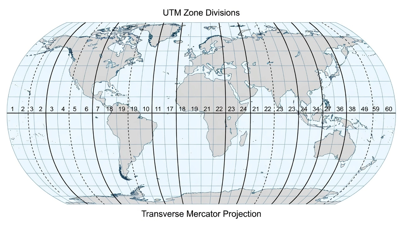
The Earth is divided into 60 UTM zones, each spanning 6 degrees of longitude in width. Zone numbering begins at the International Date Line, longitude 180° West, with Zone 1 covering 180° W to 174° W. Zones increase eastward sequentially, so Zone 2 covers 174° W to 168° W, continuing around the globe until Zone 60 completes the coverage from 174° E to 180° E. The conterminous United States falls within UTM Zones 10 through 19, with Zone 10 covering the Pacific coast from approximately 126° W to 120° W, and Zone 19 covering the northeastern states from approximately 72° W to 66° W. Major cities and their UTM zones include New York City in Zone 18, Chicago in Zone 16, Denver in Zone 13, Los Angeles in Zone 11, and Seattle in Zone 10. Europe spans Zones 28 through 38, with London near the boundary of Zone 30 and 31 (the Prime Meridian at 0° longitude falls within Zone 31), Paris in Zone 31, Berlin in Zone 33, and Rome in Zone 33. Asia spans Zones 38 through 55, with Tokyo in Zone 54 and Singapore in Zone 48. Australia spans Zones 49 through 56, with Sydney in Zone 56 and Perth in Zone 50.

Vertically, UTM zones extend from 80° South latitude to 84° North latitude. The original system was designed with limits of 80° N and 80° S, but the northern boundary was later extended to 84° N to accommodate portions of Russia and Greenland. Beyond these latitudinal limits, the Universal Polar Stereographic (UPS) projection system is employed, using two separate azimuthal projections centered on each pole. The UPS system covers all areas north of 84° N latitude (the Arctic region including the North Pole) and south of 80° S latitude (Antarctica and the surrounding Southern Ocean). This combined UTM/UPS system provides complete worldwide coverage with a consistent, standardized coordinate framework that ensures no location on Earth is left unrepresented.

Each UTM zone is further subdivided into latitude bands spanning 8 degrees of latitude, designated by letters from C to X (excluding I and O to avoid confusion with numerals 1 and 0). Band C begins at 80° S, and bands progress alphabetically northward through D, E, F, G, H, J, K, L, M, N, P, Q, R, S, T, U, V, W, and X. The X band is an exception, spanning 12 degrees of latitude (72° N to 84° N) rather than the standard 8 degrees, to accommodate the extended northern limit of the UTM system. These latitude band designations, combined with zone numbers, form the basis of the Military Grid Reference System (MGRS), a military adaptation of UTM used by NATO armed forces for operational coordination. In MGRS, a position is specified by the zone number, the latitude band letter, a 100,000-meter square identifier (two letters), and numerical easting and northing values, enabling precise position reporting with reduced digit counts.

UTM Zone Identification

Determining the correct UTM zone for a given location is a straightforward calculation based on longitude. For any longitude value expressed in degrees (treating west longitude as negative), the zone number can be computed using the formula:

Zone = floor((longitude + 180°) / 6) + 1

The result is always rounded up to the next integer value (ceiling function). For example, to find the zone for Denver, Colorado, located at approximately 105° W longitude (represented as −105°):

(−105° + 180°) = 75°

75° / 6 = 12.5

Round up to 13

Therefore, Denver, Colorado is in UTM Zone 13.

For locations east of the Prime Meridian, the same formula applies. For example, Tokyo at approximately 139° E longitude:

(139° + 180°) = 319°

319° / 6 = 53.17

Round up to 54

Therefore, Tokyo, Japan is in UTM Zone 54.

For practical field use, UTM zones are often described using both the zone number and a hemisphere designator — either “N” for north of the equator or “S” for south of the equator. For instance, “17N” indicates Zone 17 in the Northern Hemisphere, while “36S” indicates Zone 36 in the Southern Hemisphere. This distinction is critical because a given easting and northing coordinate pair can occur in both the Northern and Southern Hemisphere within the same zone, as each hemisphere has its own coordinate origin within the zone. Without the hemisphere designation, a coordinate of “500,000 mE, 5,000,000 mN” in Zone 17 could refer to a point at approximately 45° N latitude near Minneapolis, or a point at approximately 45° S latitude in the South Atlantic Ocean — two locations separated by more than 10,000 kilometers.

Useful reference points for UTM zone boundaries include:

Key Location	Approximate Longitude	UTM Zone
International Date Line (western Alaska)	180° W	Zone 1
Prime Meridian (Greenwich, UK)	0°	Zone 31
New York City	74° W	Zone 18
Chicago	87° W	Zone 16
Denver	105° W	Zone 13
Los Angeles	118° W	Zone 11
London	0°	Zone 31
Tokyo	139° E	Zone 54
Sydney	151° E	Zone 56
Moscow	37° E	Zone 37
Singapore	103° E	Zone 48

A key geometric property of the UTM zone system is that the central meridian of any UTM zone is located at the midpoint between its eastern and western boundaries. For Zone 13, which spans 108° W to 102° W, the central meridian is 105° W. For Zone 16, spanning 90° W to 84° W, the central meridian is 87° W. This central meridian is the axis along which the secant Transverse Mercator cylinder most closely approximates the Earth’s ellipsoid. The formula for calculating the central meridian of any zone is: Central Meridian = (Zone × 6) − 183 for zones in the Western Hemisphere, and Central Meridian = (Zone × 6) − 177 for zones in the Eastern Hemisphere. This central meridian defines the line of minimum scale distortion within the zone (where k = 0.9996), and it is the line along which Grid North aligns exactly with True North.

Easting and Northing

UTM coordinates are expressed as two numeric values: easting and northing, both measured in meters. This metric basis is one of the system’s primary advantages for engineering and surveying applications, as all calculations can be performed using standard Euclidean geometry without requiring spherical trigonometry. The coordinate values are always positive within their respective zones, which is achieved through the application of false origins on both axes.

Easting

The easting value (abbreviated as E or mE) represents the distance in meters east from the zone’s central meridian. To eliminate negative coordinate values for points west of the central meridian, a false easting of 500,000 meters is assigned to the central meridian itself. This means that the central meridian of any UTM zone always has an easting value of exactly 500,000 meters East (500,000 mE). Points located west of the central meridian have easting values less than 500,000 meters, while points east of the central meridian have easting values greater than 500,000 meters.

The use of false easting ensures that all coordinates within a zone are positive numbers, eliminating the sign confusion that would arise from negative coordinate values. Since the maximum width of a UTM zone at the equator is approximately 666,000 meters (6° of longitude × approximately 111 km per degree of longitude at the equator), the easternmost point in a zone can have an easting value up to about 833,000 meters (500,000 + 333,000), while the westernmost point can have an easting as low as approximately 167,000 meters (500,000 − 333,000). At higher latitudes, where lines of longitude converge dramatically, the range of easting values narrows considerably — at 60° N latitude, a degree of longitude spans only about 55.8 km, reducing the zone width to approximately 335 km, and at 84° N latitude, easting values range only from approximately 465,000 mE to 515,000 mE.

When recording UTM easting coordinates, the standard convention is to include all digits representing meters. A typical full easting coordinate might appear as 462,835 mE, meaning the point is 462,835 meters east of the false origin. To determine the point’s position relative to the central meridian, subtract 500,000: 462,835 − 500,000 = −37,165 meters, indicating the point is 37,165 meters west of the central meridian. For higher precision, decimal places are added as needed. A coordinate of 492,835.42 mE provides centimeter-level precision, with the point located 7,164.58 meters west of the central meridian.

Northing

The northing value (abbreviated as N or mN) represents the distance in meters north from the equator in the Northern Hemisphere. For the Southern Hemisphere, a different approach is used to avoid negative values: the equator is assigned a northing value of 10,000,000 meters, and coordinates decrease as one moves southward. This is known as false northing. For example, a point at 45° S latitude would have a northing of approximately 5,000,000 mN (roughly 5,000 km south of the equator), while a point at 80° S latitude would have a northing of approximately 1,100,000 mN. The 10,000,000 meter false northing ensures that all Southern Hemisphere northings remain positive over land areas — the southernmost land, at approximately 84° S in Antarctica, yields a northing of approximately 777,000 mN.

In the Northern Hemisphere, northing values range from 0 meters at the equator to approximately 9,400,000 meters at 84° N latitude. In the Southern Hemisphere, northing values range from 10,000,000 meters at the equator down to approximately 1,000,000 meters at 80° S latitude. This arrangement ensures that all northing values are positive throughout the entire UTM system without exception.

Because the same numerical northing value can exist in both hemispheres, it is essential to specify the hemisphere when communicating UTM coordinates. Northing values near 5,000,000 mN occur at approximately 45° N (near cities like Minneapolis, Milan, and Vladivostok) and also at approximately 45° S (near cities like Christchurch, New Zealand and Punta Arenas, Chile). The hemisphere is typically indicated by appending the zone number with an N or S designator (e.g., “Zone 17N” or “Zone 36S”), or by including the latitude band letter in full MGRS notation. A complete UTM coordinate is written in the format:

Zone Number + Hemisphere + Easting + Northing

For example: 18N 583,962 mE 4,506,789 mN

This coordinate identifies a location in UTM Zone 18 North, 583,962 meters east of the false origin, and 4,506,789 meters north of the equator — approximately 40.7° N latitude, 74.0° W longitude, placing it near New York City.

For the Southern Hemisphere: 36S 419,832 mE 6,234,567 mN

This identifies a location in UTM Zone 36 South, in the Southern Hemisphere.

The standard format when recording UTM coordinates for engineering inspection should follow: Zone + Easting + Northing + Datum. Example: 13N 492,835.42 4,506,789.12 (WGS84).

UTM for Distance and Area Measurement

The primary advantage of the UTM system for engineering inspection and surveying is its ability to support direct metric distance calculations using the Pythagorean theorem. Because UTM coordinates are planar Cartesian coordinates expressed in meters, the straight-line distance between any two points within the same UTM zone can be computed simply as:

d = √[(E₂ − E₁)² + (N₂ − N₁)²]

where E and N represent the easting and northing values of the two points respectively, and d is the distance in meters. This is vastly simpler than computing distances on the Earth’s curved surface using latitude and longitude, which requires great-circle distance formulas such as the Haversine formula:

d = 2R × arcsin(√[sin²((φ₂−φ₁)/2) + cos(φ₁)cos(φ₂)sin²((λ₂−λ₁)/2)])

where φ and λ represent latitude and longitude in radians, and R is the Earth’s radius (approximately 6,371 km). The Haversine formula involves trigonometric functions and requires knowing the Earth’s radius, introducing additional computation steps and potential rounding errors.

For practical inspection work, consider the following example: A pavement crack extends from UTM coordinate (489,325 mE, 4,502,100 mN) to (489,400 mE, 4,502,200 mN). The crack length is simply:

d = √[(489,400 − 489,325)² + (4,502,200 − 4,502,100)²]

d = √[(75)² + (100)²]

d = √[5,625 + 10,000]

d = √[15,625]

d = 125.0 meters

This calculation requires nothing more than basic arithmetic. Computing the same distance from latitude/longitude coordinates would require multiple trigonometric evaluations, conversion of degrees to radians, and application of the Haversine formula — a significantly more complex and error-prone process.

For area measurement, the planar nature of UTM coordinates allows direct application of standard geometric area formulas. The most commonly used method for irregular polygons is the shoelace formula (also known as Gauss’s area formula or the surveyor’s formula):

A = ½ × |Σᵢ(XᵢYᵢ₊₁ − Xᵢ₊₁Yᵢ)|

where (Xᵢ, Yᵢ) are the UTM easting (X) and northing (Y) coordinates of the polygon vertices in sequential order, and the result is in square meters. For a polygon with n vertices, the summation is performed from i = 1 to i = n, with the convention that (Xₙ₊₁, Yₙ₊₁) = (X₁, Y₁) to close the polygon.

This formula is particularly valuable in airport pavement inspection, where crack area, spall area, delamination area, and alligator cracking zones must be calculated from measured boundary coordinates. For example, a triangular spalled area with UTM vertices at (490,000, 4,505,000), (490,050, 4,505,030), and (490,020, 4,505,060) would have its area computed as:

A = ½ × |(490,000 × 4,505,030 + 490,050 × 4,505,060 + 490,020 × 4,505,000) − (4,505,000 × 490,050 + 4,505,030 × 490,020 + 4,505,060 × 490,000)|

A = ½ × |(2,207,464,700,000 + 2,208,050,703,000 + 2,207,590,200,000) − (2,207,464,700,000 + 2,207,590,200,000 + 2,208,050,703,000)|

A = ½ × 600,000 = 300,000 square meters = 300 m²

The UTM system also supports straightforward length measurement of linear features such as pavement cracks. A crack measured as a series of UTM coordinate points can have its total length computed by summing the Euclidean distances between consecutive points:

Total Length = Σⱼ√[(Eⱼ₊₁ − Eⱼ)² + (Nⱼ₊₁ − Nⱼ)²]

This method is widely used in automated pavement condition surveys where GPS-equipped inspection vehicles or UAVs collect crack location data in UTM coordinates for direct length and width calculation. Modern RTK GPS receivers can collect UTM coordinates at rates of 10-20 positions per second while the inspection vehicle travels at normal traffic speeds, generating a dense point cloud of pavement distress locations.

For airport inspection applications, ICAO Annex 14 requires accurate reporting of pavement surface condition, including crack dimensions and areas for Pavement Condition Index (PCI) determination per ASTM D5340. UTM coordinates provide the ideal framework for these measurements because all values are in meters (eliminating unit conversion errors), planar geometry simplifies area computation for irregular distress shapes, coordinates can be directly input into GIS and CAD systems for visualization, GPS receivers output coordinates directly for field validation, and multiple measurements from different inspection dates can be compared precisely over time.

{{

}}

UTM vs Geographic (Lat/Lon) for Inspection

The choice between UTM and geographic coordinates (latitude/longitude) for engineering inspection and measurement depends on the specific requirements of the task. Neither system is inherently “more accurate” — they are simply different mathematical frameworks for representing position on the Earth’s surface. The USGS explicitly states that “one system is no more or less accurate than the other. They are just two different ways of positioning a point.” However, each offers distinct advantages and disadvantages for inspection applications, and the choice significantly affects workflow efficiency and error rates.

For distance and area measurement, UTM is clearly superior. Geographic coordinates present fundamental challenges for metric measurement that make them impractical for direct engineering calculations:

Variable degree length. One degree of longitude does not represent a fixed distance. At the equator, 1° of longitude equals approximately 111,320 meters, but at 60° N latitude, 1° of longitude equals only about 55,800 meters, and at 80° N latitude, it is merely 19,400 meters. This variable relationship makes direct distance calculation from latitude/longitude differences impossible without complex spherical trigonometry. One degree of latitude is more consistent, varying from approximately 110,574 meters at the equator to 111,694 meters at the poles, but the nonlinear relationship between latitude, longitude, and actual distance on the Earth’s surface remains a fundamental obstacle to simple metric calculations.

Trigonometric distance formulas. The Haversine formula, Vincenty’s formula, or spherical law of cosines must be used to compute even simple distances between points in geographic coordinates. Vincenty’s formula provides higher accuracy than Haversine by modeling the Earth as an oblate spheroid rather than a sphere, but it requires iterative solutions and is computationally intensive — typically requiring 2-4 iterations for convergence to 0.5 mm precision. These formulas are significantly more computationally intensive and error-prone than the simple Pythagorean calculation possible with UTM.

Complex area calculation. Computing the area of a polygon defined by geographic coordinates requires integration over the Earth’s curved surface, using formulas that account for latitude-dependent convergence of meridians. The spherical polygon area formula involves summing spherical excess values for each triangle in the polygon, requiring conversion of all coordinates to three-dimensional Cartesian vectors and computing angles between great-circle arcs.

Inconsistent units. Latitude and longitude are measured in degrees, minutes, and seconds (or decimal degrees), while the distances they represent vary with location. Converting to linear units (meters, feet) adds conversion steps and potential error sources. The conversion factor between a degree of longitude and meters changes continuously with latitude, requiring trigonometric calculations for even the simplest unit conversions.

For positional reference and global navigation, geographic coordinates have distinct advantages. They provide a universal, unambiguous reference that works anywhere on Earth without zone boundaries. Latitude/longitude is the international standard for aviation navigation (ICAO Annex 2 — Rules of the Air), maritime operations (IMO SOLAS convention), and global scientific research. All GPS receivers natively output geographic coordinates in WGS84 datum as their default coordinate format, and no zone selection or boundary crossing issues exist.

For airport pavement inspection, UTM coordinates are strongly preferred for several specific applications:

Crack Length Measurement. A longitudinal crack running 50 meters along a runway can be measured by simply differencing the northing coordinates of its start and end points (for north-south oriented cracks) or by applying the Pythagorean theorem for diagonally oriented cracks. The result is immediately in meters with no additional calculations required.

Distressed Area Reporting. Spalled areas, potted sections, or alligator-cracked zones measured in UTM coordinates can have their areas computed directly in square meters using the shoelace formula without any projection or conversion steps. This is essential for generating ICAO-compliance reports per Annex 14 specifications, where pavement repair quantities must be estimated in square meters.

Line-of-Sight Distance. For obstacle clearance surfaces and approach path assessments per ICAO Annex 14, Volume I, Chapter 4, three-dimensional distances combining horizontal UTM distance and vertical elevation difference are computed as: d₃D = √[(ΔE)² + (ΔN)² + (ΔH)²] where ΔE and ΔN are UTM coordinate differences and ΔH is elevation difference in meters.

Coordinate Repeatability. When conducting recurring inspections (e.g., annual pavement condition surveys as required by FAA Advisory Circular 150/5380-6C), returning to the same crack or distress location is straightforward when UTM coordinates are recorded. The metric coordinates can be loaded into a GPS receiver for direct navigation back to the exact inspection point, enabling precise temporal monitoring of crack propagation rates and deterioration trends.

UTM and GPS

The Global Positioning System (GPS) and the UTM coordinate system are complementary technologies that serve different but interconnected purposes in spatial data collection. GPS receivers fundamentally compute positions in Earth-Centered, Earth-Fixed (ECEF) Cartesian coordinates (X, Y, Z in meters from the Earth’s center of mass), which are then transformed into geographic coordinates (latitude, longitude, ellipsoidal height) referenced to the WGS84 datum — the World Geodetic System 1984, which is the standard reference frame for GPS established by the United States Department of Defense. The WGS84 datum defines the size and shape of the Earth through its reference ellipsoid with a semi-major axis of 6,378,137.0 meters and an inverse flattening of 298.257223563.

Most GPS receivers and mapping software can convert these WGS84 geographic coordinates to UTM coordinates in real time through an onboard projection engine. The conversion process applies the Transverse Mercator projection formulas to the WGS84 ellipsoid parameters, producing easting and northing values for the appropriate UTM zone. Users can typically select UTM coordinate display in their GPS receiver’s setup menu under a “Coordinate System” or “Grid” option, after which the receiver automatically determines the correct zone based on the current longitude and displays coordinates in that zone. As the user moves across zone boundaries, modern GPS receivers automatically switch to the adjacent zone or optionally display coordinates in both zones simultaneously.

For survey-grade GPS applications used in airport inspection, the relationship between GPS and UTM is particularly critical:

Real-Time Kinematic (RTK) GPS achieves centimeter-level positioning accuracy by using base station corrections transmitted via radio link or cellular network to the rover receiver. A modern RTK GPS receiver can output UTM easting and northing coordinates with 1-2 cm horizontal accuracy under favorable conditions (open sky view, good satellite geometry, base station within 10-20 km). This level of precision is sufficient for crack width measurement, joint faulting assessment, and pavement roughness profiling.

Post-Processed Kinematic (PPK) GPS offers even higher precision by recording raw satellite observations in the field and processing them after the survey using base station data from a permanent CORS (Continuously Operating Reference Station) network. PPK processing can achieve sub-centimeter UTM coordinate accuracy, suitable for deformation monitoring, settlement measurement, and precision pavement profiling.

Differential GPS (DGPS) provides meter-level UTM accuracy (typically 1-3 meters) using correction signals from coastal beacon stations or satellite-based augmentation systems (SBAS such as WAAS, EGNOS, MSAS). This accuracy level is suitable for locating pavement distress for subsequent detailed inspection, mapping pavement feature boundaries, and general navigation to inspection points.

When using GPS for UTM coordinate collection in airport environments, specific protocols must be followed:

Always verify the datum. Ensure the GPS receiver is set to WGS84 before any coordinate conversion. Using the wrong datum — such as NAD83 (North American Datum 1983), ED50 (European Datum 1950), or local datums — can introduce position errors of 1-200 meters depending on location and the datum transformation parameters. In North America, NAD83 and WGS84 are essentially identical for most practical purposes (differences of less than 2 meters), but in other regions, datum differences can be substantial.

Check the UTM zone. GPS receivers typically auto-select the UTM zone based on longitude, but when working near zone boundaries (within approximately 0.5° of the zone edge), manual confirmation is recommended to avoid incorrect zone assignment. Some receivers allow display of dual-zone coordinates for boundary areas.

Record the zone with coordinates. Always include the UTM zone number and hemisphere with every coordinate pair. A coordinate of “583,962 mE, 4,506,789 mN” without zone and hemisphere is ambiguous and effectively meaningless for data archival purposes.

Consider elevation effects. UTM provides only horizontal positioning (easting and northing). Vertical position must be handled separately, typically using ellipsoidal height from GPS (measured relative to the WGS84 ellipsoid) or orthometric height from geoid models (measured relative to mean sea level). The difference between ellipsoidal height and orthometric height, known as the geoid undulation, can vary by ±100 meters globally and must be accounted for when converting between height systems for airport elevation reporting per ICAO Annex 14 requirements.

Converting Lat/Lon to UTM

The conversion from geographic coordinates (latitude φ, longitude λ) to UTM coordinates (easting E, northing N) involves a series of mathematical operations based on the Transverse Mercator projection applied to the reference ellipsoid. The full derivation is complex, involving integration of the meridian distance formula and series expansions for the ellipsoidal corrections. The core conversion parameters are defined by the International Association of Geodesy (IAG) and the International Federation of Surveyors (FIG) and are implemented in all major GIS and surveying software packages.

Basic Conversion Parameters

Parameter	Symbol	WGS84 Value	Description
Semi-major axis	a	6,378,137.0 m	Equatorial radius of Earth
Inverse flattening	1/f	298.257223563	Ellipsoid flattening ratio
Eccentricity squared	e²	0.00669437999014	Ellipsoid eccentricity
Scale factor at central meridian	k₀	0.9996	UTM scale factor
False easting	FE	500,000 m	Easting at central meridian
False northing (North)	FN	0 m	Northing at equator (NH)
False northing (South)	FN	10,000,000 m	Northing at equator (SH)

The Conversion Process

Step 1: Determine the UTM zone. Zone = floor((λ + 180°) / 6) + 1, where λ is in degrees (west longitude negative).

Step 2: Calculate the central meridian. For the zone determined in Step 1, the central meridian is λ₀ = (Zone × 6) − 183° for zones in the Western Hemisphere. In simplified form: λ₀ = 6° × (Zone − 30) − 3° for east longitude, or alternatively, central meridian = (Zone × 6 − 3)° — 180° for Western Hemisphere zones.

Step 3: Compute meridian distance. The distance from the equator to the latitude φ along the ellipsoid is calculated using the series expansion:

M = a × [(1 − e²/4 − 3e⁴/64 − 5e⁶/256 …) × φ − (3e²/8 + 3e⁴/32 + 45e⁶/1024 …) × sin(2φ) + (15e⁴/256 + 45e⁶/1024 …) × sin(4φ) − (35e⁶/3072 …) × sin(6φ) + …]

Step 4: Compute the northing. For the Northern Hemisphere: N = k₀ × M. For the Southern Hemisphere: N = k₀ × M + 10,000,000 m.

Step 5: Compute the easting. E = FE + k₀ × a × (λ − λ₀) × cos(φ) + higher-order terms, where the higher-order terms include corrections for the ellipsoidal convergence of meridians and the curvature of the projection.

Practical Conversion Tools

The NOAA National Geodetic Survey (NGS) Coordinate Conversion and Transformation Tool (NCAT) provides authoritative conversion between geographic coordinates and UTM for the United States. The tool supports WGS84, NAD83, and other datums, outputting UTM easting and northing with configurable decimal precision. It uses NADCON for datum transformations and provides rigorous error estimates for each conversion.

For international use, the United States National Geospatial-Intelligence Agency (NGA) provides Geotrans libraries that implement the precise UTM conversion formulas for all standard ellipsoids, including WGS84, GRS80, Clarke 1866, Bessel 1841, Hayford 1909, and many others. The libraries are available in C++, Java, and Python and are used by NATO, allied military forces, and civilian mapping agencies worldwide.

When converting coordinates for inspection work, maintain consistent precision based on the required measurement accuracy:

Required Accuracy	Decimal Places in UTM	Typical Use
1 meter	0 decimal places (whole meters)	General navigation, distress location
0.1 meter	1 decimal place	Approach surveys, crack zone mapping
0.01 meter	2 decimal places	Detailed crack measurement
0.001 meter	3 decimal places	Precision engineering, forensic analysis

UTM Distortion at Zone Edges

The UTM system, like all map projections, involves inherent scale distortion — the inevitable mathematical consequence of representing a curved surface (the Earth) on a flat plane. Understanding this distortion is critical for inspection work, particularly when measurements are taken near zone boundaries or when high-accuracy requirements exceed 1:2,500.

The UTM projection is a secant Transverse Mercator projection, meaning the projection cylinder intersects the Earth’s ellipsoid along two lines parallel to the central meridian rather than being tangent along a single line. These two lines of intersection — located approximately 180 km east and west of the central meridian — are lines of exact scale, where the scale factor equals exactly 1.00000 (no distortion). Between these lines, distances on the grid are slightly shorter than true ground distances; outside these lines, grid distances are slightly longer.

Scale Factor Characteristics

The scale factor k in UTM varies continuously across the width of each zone according to a well-defined mathematical relationship:

Location from Central Meridian	Scale Factor (k)	Effect on Measured Distance
0 km (central meridian)	0.9996	Grid distance is 0.04% shorter than true ground
~90 km east or west	0.9998	Grid distance is 0.02% shorter
~180 km east or west	1.00000	Exact scale — no distortion
~270 km east or west	1.0005	Grid distance is 0.05% longer
~333 km (zone edge, ~3°)	~1.0010	Grid distance is ~0.10% longer

The scale factor at any point within a UTM zone can be computed from the transverse Mercator projection formulas. For most practical purposes, the scale factor at a given longitude offset from the central meridian is approximately:

k = k₀ × sec(Δλ × cos(φ))

where Δλ is the angular distance from the central meridian (in radians), φ is the latitude, and k₀ = 0.9996. A more precise calculation includes terms for the ellipsoidal eccentricity and the curvature of the transverse Mercator projection.

For a 100-meter distance measured on the UTM grid at the central meridian, the true ground distance is 100.04 meters (100 / 0.9996). The same grid distance of 100 meters at the zone edge (k ≈ 1.0010) corresponds to a true ground distance of 99.90 meters (100 / 1.0010). The difference of 14 cm over 100 meters may be negligible for general pavement inspection but could be significant for precision alignment and high-accuracy crack width monitoring.

Grid Convergence

In addition to scale distortion, UTM coordinates also exhibit grid convergence γ (gamma) — the angular difference between Grid North (the direction of the UTM grid’s north-south lines, which are parallel to the central meridian) and True North (the direction of meridians converging at the geographic North Pole). Grid convergence varies from zero at the central meridian to a maximum at the zone edges, calculated as:

γ = Δλ × sin(φ)

where Δλ is the longitude difference from the central meridian. Grid convergence reaches approximately 0.5° at the zone edge at the equator, approximately 2.6° at 60° latitude, and approximately 3.0° at 84° latitude. For inspection measurements, grid convergence affects directional measurements (bearings) but does not affect distance or area calculations within the same zone. Surveyors using UTM for airport work must account for convergence when converting between grid bearings and true bearings for obstacle clearance surfaces (ICAO Annex 14, Chapter 4) and approach path alignment calculations.

Practical Implications for Inspection

Within a single zone — the most common case for airport work — distortion effects are relatively small. The maximum scale error is approximately 0.04% at the central meridian and approximately 0.10% at the zone edges. For a runway 3,000 meters in length, the maximum scale-related error is approximately 1.2 to 3.0 meters depending on its position within the zone. For most pavement inspection tasks (crack mapping, distress area quantification, PCI surveys), this level of distortion is acceptable. However, for high-precision work — such as measuring crack widths to sub-millimeter accuracy, monitoring joint movements, or performing deformation analysis — scale corrections should be applied using the formula: True Distance = Grid Distance / Scale Factor.

When working near zone boundaries, airports located within approximately 30 km of a UTM zone edge may encounter situations where an airport’s runways or infrastructure span two adjacent UTM zones. In such cases, practical strategies include:

• Using the exact scale factor at the airport’s reference point to correct all measurements within that zone
• Employing a Modified Transverse Mercator (MTM) projection with a central meridian optimized for the specific airport location, reducing the maximum distortion by recentering the zone
• Using geographic coordinates for position storage and computing distances with Vincenty’s formula, then converting to UTM only for reporting
• Cross-zone averaging with a common central meridian for the project area, effectively creating a local grid system for the airport
• Using the UTM zone that covers the majority of the airport’s area and converting any points in the secondary zone to the primary zone’s reference frame using rigorous coordinate transformation

The USGS recommends that UTM be used with awareness of its distortion characteristics, applying scale corrections when measurement accuracy requirements exceed 1:2,500 (approximately 4 cm per 100 m). For most airport pavement inspection applications, standard UTM coordinates without scale correction provide adequate accuracy for pavement condition assessment and repair quantity estimation.

{{

}}

WGS84 UTM

WGS84 (World Geodetic System 1984) is the geodetic datum that forms the foundation for GPS positioning and, by extension, for most modern UTM coordinate applications. The relationship between WGS84 and UTM is defined by the application of the Transverse Mercator projection to the WGS84 ellipsoid parameters. ICAO mandates the use of WGS84 for all aeronautical positioning and navigation applications, as specified in ICAO Annex 4 — Aeronautical Charts and ICAO Annex 15 — Aeronautical Information Services. This mandate ensures global interoperability of aeronautical data, including airport coordinates, navigation aid positions, and obstacle locations.

The WGS84 Ellipsoid Parameters

The WGS84 ellipsoid, which defines the shape of the Earth for UTM projection calculations, has the following defining parameters:

Parameter	Symbol	Value	Unit
Semi-major axis	a	6,378,137.0	meters
Inverse flattening	1/f	298.257223563	dimensionless
Semi-minor axis	b	6,356,752.3142	meters
Eccentricity squared	e²	0.00669437999014	dimensionless
Angular velocity	ω	7,292,115.0 × 10⁻¹¹	rad/s
Earth’s gravitational constant	GM	3,986,004.418 × 10⁸	m³/s²

When converting WGS84 geographic coordinates to UTM, the Transverse Mercator projection uses these ellipsoid parameters to compute the easting and northing values. The result is a WGS84 UTM coordinate — a UTM coordinate derived from WGS84 datum positions. The WGS84 datum is revised periodically through “realizations” — sets of coordinates for reference stations that refine the datum’s accuracy. The major realizations include WGS84 (G730), WGS84 (G873), WGS84 (G1150), and WGS84 (G1762), with each successive realization improving the alignment with the International Terrestrial Reference Frame (ITRF). For practical inspection work, these differences are negligible (less than 5 cm globally).

UTM and Other Datums

UTM coordinates can be computed on any reference ellipsoid, not only WGS84. Historically, UTM was implemented on various local ellipsoids before the adoption of global reference systems. The critical point is that the datum must be specified alongside UTM coordinates for them to be unambiguous:

WGS84 UTM: UTM derived from WGS84 positions (the global standard for GPS, used by ICAO, FAA, and all modern aeronautical applications). This is the recommended datum for all airport inspection work.

NAD83 UTM: UTM derived from North American Datum 1983 (used by USGS for topographic maps, federal agencies, and state surveying programs in the United States). NAD83 is virtually identical to WGS84 for most practical purposes, with differences of less than 2 meters in the conterminous US. However, at the centimeter level of precision achievable with modern RTK GPS, the datum difference must be accounted for using NADCON transformation grids.

ED50 UTM: UTM derived from European Datum 1950 (historically used in Western Europe before the adoption of ETRS89/WGS84). ED50 UTM can differ from WGS84 by up to 200 meters in some locations due to the use of the International 1924 (Hayford) ellipsoid with a different center relative to the Earth’s center of mass.

Clarke 1866 UTM: Used on older USGS topographic maps and in historical engineering surveys, particularly in North America. Clarke 1866 UTM coordinates can differ from WGS84 by up to 200 meters in some locations.

GRS80 UTM: The Geodetic Reference System 1980 ellipsoid is nearly identical to WGS84 (the semi-major axis differs by less than 0.1 mm), and GRS80 UTM coordinates are essentially interchangeable with WGS84 UTM at all practical levels of precision.

For ICAO-compliant airport inspection and mapping, WGS84 must be used as the reference datum per ICAO Annex 4, Annex 15, and ICAO Doc 9674 (World Geodetic System — 1984 (WGS84) Manual). This ensures that airport coordinates, runway thresholds, navigation aid positions, and obstacle locations are globally consistent and interoperable across national boundaries and between different aviation authorities and service providers.

UTM in TarmacView Mapping

TarmacView integrates the UTM coordinate system as a primary spatial reference for airport pavement inspection and mapping applications. The use of UTM within the TarmacView platform enables precise metric measurement of pavement distress features, including crack length, crack width, spalled area, alligator cracking zones, joint spalling, patching deterioration, and surface delamination extents, all quantifiable in standard metric units that align with international reporting requirements.

How TarmacView Uses UTM

When inspection data is collected using GPS-equipped devices — including UAVs (drones) with RTK GPS, specialized pavement inspection vehicles with integrated GNSS receivers, or handheld survey-grade GPS units — TarmacView processes the raw GPS positions in WGS84 geographic coordinates and converts them to UTM coordinates using rigorous geodetic transformations based on the Transverse Mercator projection formulas applied to the WGS84 ellipsoid. The conversion is performed internally within the TarmacView platform, ensuring consistent and traceable coordinate transformations across all inspection sessions.

Measurement Computation. All crack lengths, polygon areas, and linear distances are computed using UTM planar geometry. For a longitudinal crack on Runway 09/27, TarmacView extracts the easting and northing coordinates of the crack’s start and end points at millimeter precision from the GPS-inertial positioning system. The Euclidean distance calculation provides an accurate metric length in meters that can be directly reported in ICAO-compliant inspection documentation, including the Airport Pavement Condition Index (PCI) report per ASTM D5340 and FAA Advisory Circular 150/5380-6C.

Area Calculation for Distress Polygons. When an inspector delineates a spalled area, alligator-cracked zone, or patching boundary, TarmacView captures the UTM coordinates of the polygon vertices at the resolution of the GPS data (typically 1-2 cm with RTK GPS). The shoelace formula computes the enclosed area in square meters. This area value is essential for quantifying pavement repair quantities (cubic meters of patching material required), estimating material requirements for partial-depth repairs, tracking deterioration progression over time (e.g., a spall that grew from 0.5 m² to 1.2 m² over 12 months), and generating cost estimates for pavement rehabilitation programs.

Multi-Zone Handling. For airports spanning large geographic areas — such as major international hubs with multiple runways exceeding 10 km in total length — TarmacView automatically manages UTM zone assignments, ensuring that coordinates are correctly referenced regardless of the airport’s location relative to zone boundaries. When an airport lies near a zone boundary, TarmacView applies a consistent zone across the entire facility using coordinate transformations for any points falling in adjacent zones.

Cross-Visit Comparison. UTM coordinates provide a stable, repeatable reference frame for comparing inspection results across different survey dates. A longitudinal crack measured at UTM coordinates E 492,835.42, N 4,506,789.12 during a January inspection can be precisely re-visited during the July inspection using the same coordinates loaded into a GPS receiver for navigation. The coordinate differences between inspections yield crack propagation rates in millimeters per month, enabling data-driven maintenance prioritization based on the rate of deterioration.

Integration with GIS and CAD. UTM-based inspection data from TarmacView can be exported directly to GIS platforms (ArcGIS, QGIS, MapInfo) and CAD software (AutoCAD, MicroStation, Bricscad) for integration with airport master plans, pavement management systems (PMS), and infrastructure asset databases. The UTM coordinate system is natively supported by all major GIS and CAD platforms, eliminating the need for coordinate conversion when transferring data between systems.

Practical Benefits for Airport Inspection

The use of UTM in TarmacView provides concrete, measurable advantages for airport pavement inspection operations:

Metric consistency. All coordinates and measurements are in meters or square meters, eliminating unit conversion errors between field measurement and reporting. No conversion factors or unit transformations are required at any stage of the inspection workflow.

Direct area quantification. Polygon areas are computed in square meters directly from UTM coordinates using the shoelace formula, without requiring complex spherical geometry or area correction factors. The area calculation is exact for the planar coordinates and provides accuracy within the scale factor tolerance of the UTM projection.

Longitudinal monitoring. Crack growth rates, spall expansion velocities, and deterioration progression are calculated by comparing UTM coordinates across successive inspection dates. A crack that extended from coordinate E 492,635.12 to E 492,636.48 between inspections has grown by 1.36 meters, measurable directly from the coordinate differences.

Regulatory compliance. ICAO Annex 14 requirements for accurate pavement condition reporting, FAA Advisory Circular standards for PCI surveys, and national aviation authority requirements for aerodrome certification are satisfied through UTM-based measurement traceability.

Interoperability. Inspection data can be shared seamlessly with engineering consultants (who standardize on UTM for airport design work), regulatory agencies (who require WGS84 positions for aeronautical data), and construction contractors (who use UTM for quantity take-offs and construction layout).

TarmacView’s implementation of UTM follows the WGS84 datum standard as mandated by ICAO for all aeronautical data, ensuring that inspection coordinates are globally consistent and compatible with official aerodrome mapping requirements defined in ICAO Annex 4 (Aeronautical Charts), ICAO Annex 15 (Aeronautical Information Services), and ICAO Doc 9674 (World Geodetic System — 1984 (WGS84) Manual). This compliance ensures that all pavement inspection data collected through TarmacView meets the rigorous standards required for international aerodrome certification.

Summary

The Universal Transverse Mercator (UTM) coordinate system provides a globally standardized, metric-based plane coordinate grid that is indispensable for surveying, engineering, airport pavement inspection, and mapping applications. By dividing the Earth into 60 zones, each 6 degrees of longitude wide, UTM transforms the challenge of working on a curved Earth into a manageable planar coordinate problem with easting and northing values in meters. The system’s adoption by NATO, USGS, national mapping agencies worldwide, and the global surveying profession attests to its effectiveness as a universal coordinate framework for large-scale spatial measurement.

Key advantages of UTM for inspection work include direct Euclidean distance calculation (Pythagorean theorem), planar area measurement using the shoelace formula, compatibility with GPS technology through the WGS84 datum, seamless integration with GIS and CAD platforms, and a standard metric unit system that eliminates conversion errors. While UTM introduces scale distortion ranging from 0.9996 at the central meridian to approximately 1.0010 at zone edges, these effects are well-understood, mathematically predictable, and correctable for high-precision applications using established scale factor formulas.

For airport pavement inspection, TarmacView leverages UTM to provide accurate, repeatable, and ICAO-compliant measurements of crack lengths, distressed areas, and pavement deterioration features, enabling effective infrastructure management and maintenance planning. The combination of GPS positioning technology, the WGS84 datum, and the UTM coordinate grid creates a powerful framework for precision measurement of airport infrastructure — from runway crack monitoring to comprehensive pavement condition assessment — supporting the safety, efficiency, and regulatory compliance of aviation operations worldwide.